Mathematical Statistics

Random Variables, Random Sampling, and Chapter 2 in Review

Samir Orujov, PhD

ADA University, School of Business

Information Communication Technologies Agency, Statistics Unit

2026-09-23

🎯 Learning Objectives

By the end of this lecture, you will be able to:

  • Define a random variable as a real-valued function on \(S\) (Definition 2.12) — load-bearing

  • Compute \(P(Y = y)\) by summing the probabilities of the sample points in \(\{Y = y\}\)load-bearing

  • Count the \(\binom{N}{n}\) possible simple random samples and show each unit is included with probability \(n/N\)

  • Choose the right Chapter 2 tool for a problem, and combine several in one calculation

The first two carry all of Chapter 3. Sampling and the summary we meet more briefly.

🗺️ Where We Are

Wackerly §§2.11–2.13

Last class ended: turning outcomes into numbers — random variables, random sampling, and a synthesis of Chapter 2.

A bank’s risk committee holding three SME loans does not ask which loans default. It asks how many, and how much money is lost.

Those are numbers, not lists of outcomes. Today we build the bridge from a sample space to a number — and from there, in Chapter 3, to a distribution.

📐 Definition 2.12: Random Variable

Definition 2.12 (Wackerly §2.11)

A random variable is a real-valued function for which the domain is a sample space.

So \(Y\) takes each sample point \(E_i \in S\) to a number \(Y(E_i)\). Several points may share a value; no point gets two.

The numerical event \(\{Y = y\}\) is the set of all sample points assigned the value \(y\). These sets partition \(S\): they are mutually exclusive, and together they cover it.

🏦 Three SME Loans

A Baku bank holds three loans that default independently: construction, \(P = 0.10\); retail, \(P = 0.05\); agriculture, \(P = 0.20\). Let \(Y\) = number of defaults.

Sample point Probability \(Y\)
NNN \(0.9 \times 0.95 \times 0.8 = 0.684\) 0
DNN, NDN, NND \(0.076,\ 0.036,\ 0.171\) 1
DDN, DND, NDD \(0.004,\ 0.019,\ 0.009\) 2
DDD \(0.1 \times 0.05 \times 0.2 = 0.001\) 3

The points are not equally likely, so we cannot count — we must sum.

➕ From Sample Points to \(P(Y = y)\)

\(P(Y = y)\) is the sum of the probabilities of the sample points assigned the value \(y\).

\[P(Y = 1) = P(\text{DNN}) + P(\text{NDN}) + P(\text{NND}) = 0.076 + 0.036 + 0.171 = 0.283\]

\[P(Y = 0) = 0.684, \quad P(Y = 2) = 0.032, \quad P(Y = 3) = 0.001\]

The four values sum to 1, because the events \(\{Y = y\}\) partition \(S\). That check is free — always make it.

💻 The Same Calculation in R

p  <- c(construction = 0.10, retail = 0.05, agriculture = 0.20)
S  <- expand.grid(c1 = 0:1, c2 = 0:1, c3 = 0:1)          # 8 sample points
S$prob <- apply(S, 1, function(d) prod(ifelse(d == 1, p, 1 - p)))
S$Y    <- rowSums(S[, 1:3])                             # the function Y(E_i)
pY <- tapply(S$prob, S$Y, sum)                           # sum within {Y = y}
round(pY, 3); sum(pY)
    0     1     2     3 
0.684 0.283 0.032 0.001 
[1] 1
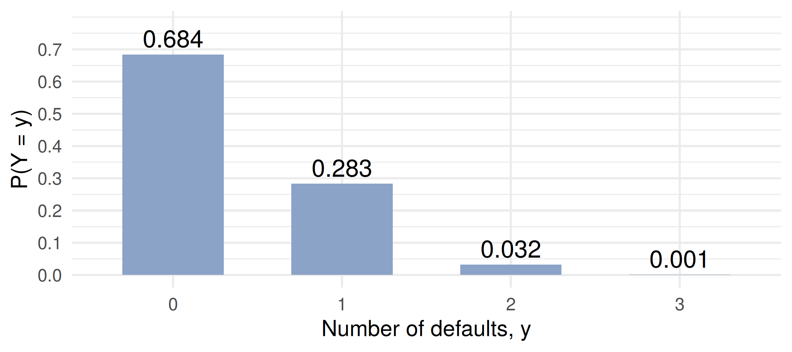

📊 The Picture: \(P(Y = y)\)

Eight sample points collapsed into four numbers. In Chapter 3 this list of values gets a name: the probability distribution of \(Y\).

💰 A Second Function on the Same \(S\)

Exposures are 200, 150 and 100 thousand AZN. Let \(L\) = loss in default (thousand AZN).

NNN NND NDN DNN NDD DND DDN DDD
0 100 150 200 250 300 350 450

Same experiment, same \(S\), a different function — and a different partition: every point gets its own value.

\(P(L \ge 250) = 0.009 + 0.019 + 0.004 + 0.001 = 0.033\). Here \(\{L \ge 250\} = \{Y \ge 2\}\) exactly: it is one set of sample points, described by two random variables.

🎲 §2.12: The Design Matters

A statistical experiment observes a sample from a population, and uses the probability of the observed sample to make an inference. So the sampling method — the design — must be stated.

An auditor picks \(n = 2\) of a bank’s \(N = 5\) branches. Probability of drawing one specific pair \(\{a, b\}\):

  • Without replacement: \(\binom{5}{2} = 10\) equally likely pairs, so \(1/10\).
  • With replacement: 25 equally likely ordered draws; \(\{a, b\}\) arises as \((a, b)\) or \((b, a)\), so \(2/25\).

📐 Definition 2.13: Random Sample

Definition 2.13 (Wackerly §2.12)

Let \(N\) and \(n\) be the numbers of elements in the population and sample. If the sampling is conducted so that each of the \(\binom{N}{n}\) samples has an equal probability of being selected, the sampling is random, and the result is a random sample.

Each sample therefore has probability \(1 / \binom{N}{n}\). In practice the draw is made by software — or, in the book, from a random number table (Table 12, Appendix 3).

🏛️ Worked Example: A Branch Audit

The Central Bank audits a simple random sample of \(n = 6\) of a commercial bank’s \(N = 30\) branches.

Number of possible samples: \(\binom{30}{6} = 593{,}775\), each with probability \(1/593{,}775\).

Is the Ganjlik branch audited? Count the samples containing it: fix it, choose the other 5 from 29. \[P(\text{included}) = \frac{\binom{29}{5}}{\binom{30}{6}} = \frac{6}{30} = 0.2 = \frac{n}{N}\]

Every branch faces the same \(n/N\). That is the sense in which an SRS is “fair”.

💻 Checking \(n/N\) by Simulation

N <- 30; n <- 6
choose(N, n)                                   # number of possible samples
[1] 593775
audits <- replicate(20000, sample(1:N, n))     # 20,000 simple random samples
incl <- sapply(1:N, function(b) mean(colSums(audits == b)))  # share containing b
round(range(incl), 3)                          # every branch near n/N = 0.2
[1] 0.195 0.205

Each of the 30 branches was audited in about 20% of the simulated samples.

🏘️ Not Every Survey Is One SRS

A household budget survey needs 800 households across Azerbaijan. One SRS could, by pure chance, draw them mostly from Baku.

Instead: allot a number of households to each region, and draw an SRS within each region. The pieces are then combined.

Such designs are only partially random, and are a course in themselves. For us, Definition 2.13 is the building block — and the random variables of Chapter 3 will be defined on its sample space.

🧠 Think-Pair-Share

A survey firm interviews an SRS of \(n = 3\) of the \(N = 10\) households on one street. Four of the ten hold a bank loan.

Four minutes, in pairs:

  1. How many different samples are possible?

  2. What is the probability that a given household is interviewed?

  3. Let \(Y\) = number of indebted households in the sample. Find \(P(Y = 0)\) and \(P(Y = 2)\).

✅ Think-Pair-Share: Solution

  1. \(\binom{10}{3} = 120\) samples, each with probability \(1/120\).

  2. \(\binom{9}{2}/\binom{10}{3} = 36/120 = 3/10 = n/N\).

  1. \(Y\) is a random variable on the 120-point sample space. Count the points in each event: \[P(Y = 0) = \frac{\binom{6}{3}}{120} = \frac{20}{120} = 0.167, \qquad P(Y = 2) = \frac{\binom{4}{2}\binom{6}{1}}{120} = \frac{36}{120} = 0.3\]

Equally likely points, so here summing is counting.

🧭 §2.13: Which Tool, When?

The problem gives you Reach for
A small \(S\) you can list Sample-point method (§2.5)
Equally likely points, too many to list Counting rules (§2.6)
“Given that …”, or a two-way table Conditional probability (§2.7)
“Unrelated”, “separately” Independence: multiply (§2.7)
“Both” / “either” / “at least one” Multiplicative, additive laws, complement (§2.8)
A compound event to decompose Event-composition method (§2.9)
Stages or states, then a reversal Total probability, Bayes (§2.10)

🔗 Synthesis: Up-Days on an Index

A stock index is in a calm regime with probability 0.7, volatile with 0.3. Given the regime, days are independent: \(P(\text{up}) = 0.6\) if calm, \(0.4\) if volatile. Let \(Y\) = number of up-days in the next 3 trading days.

Given calm (independence, then counting the \(\binom{3}{y}\) orderings): \[P(Y = 3 \mid \text{calm}) = 0.6^3 = 0.216, \qquad P(Y = 3 \mid \text{volatile}) = 0.4^3 = 0.064\]

Total probability over the two regimes: \[P(Y = 3) = 0.7(0.216) + 0.3(0.064) = 0.1512 + 0.0192 = 0.1704\]

🔗 Synthesis: Reading the Regime Back

Bayes’ rule: three up-days in a row — how sure are we the market is calm? \[P(\text{calm} \mid Y = 3) = \frac{0.1512}{0.1704} = 0.887\]

y <- 0:3
calm <- choose(3, y) * 0.6^y * 0.4^(3 - y)     # P(Y = y | calm): orderings x product
vol  <- choose(3, y) * 0.4^y * 0.6^(3 - y)     # P(Y = y | volatile)
pY   <- 0.7 * calm + 0.3 * vol                 # total probability
out  <- rbind(P_Y = round(pY, 4), P_calm_given_Y = round(0.7 * calm / pY, 3))
colnames(out) <- paste0("y=", y); out
                  y=0    y=1    y=2    y=3
P_Y            0.1096 0.3312 0.3888 0.1704
P_calm_given_Y 0.4090 0.6090 0.7780 0.8870

Prior 0.7, posterior 0.887 after three up-days — and 0.409 after none.

📝 Quiz #1: Summing Sample Points

Two bond coupons are due; each is paid with probability 0.9, independently. \(Y\) = number of missed coupons. What is \(P(Y = 1)\)?

  • \(0.18\)
  • \(0.09\)
  • \(0.10\)
  • \(0.81\)

📝 Quiz #2: Inclusion Probability

A compliance officer draws an SRS of 5 client files from 40. What is the probability that a particular client’s file is drawn?

  • \(1/40\)
  • \(1/\binom{40}{5}\)
  • \(5/40 = 0.125\)
  • \(5/39\)

📝 Quiz #3: What Is a Random Variable?

A loan is observed for one year. Which of these is a random variable?

  • The event that the loan defaults
  • The sample space \(\{\text{default}, \text{no default}\}\)
  • The number of defaults: 1 if it defaults, 0 if not
  • The probability of default, 0.08

📋 Key Formulas

Statement
Definition 2.12 \(Y: S \to\) the real line
numerical event \(\{Y = y\} = \{E_i \in S : Y(E_i) = y\}\)
probability of a value \(P(Y = y) = \sum_{E_i:\, Y(E_i) = y} P(E_i)\)
the check \(\sum_y P(Y = y) = 1\)
Definition 2.13 each of \(\binom{N}{n}\) samples has probability \(1/\binom{N}{n}\)
inclusion probability \(\binom{N-1}{n-1} / \binom{N}{n} = n/N\)

📋 Summary

  • A random variable is a function on \(S\); the events \(\{Y = y\}\) partition \(S\)

  • \(P(Y = y)\) is a sum over sample points — a count only when they are equally likely

  • One \(S\) carries many random variables: defaults, losses, up-days

  • An SRS makes all \(\binom{N}{n}\) samples equally likely, so each unit is included with probability \(n/N\)

  • Chapter 2 is a toolbox; hard problems use several tools in sequence

📚 Practice Problems

Wackerly, 7th edition

  • §2.11: exercises 2.139 – 2.142; supplementary 2.150, 2.167, 2.170

  • Chapter 2 supplementary exercises for review: 2.146, 2.149, 2.152, 2.157, 2.173, 2.174

Week 5, Problem Set 1 opens today and closes 17 October at 23:59 on WeBWorK, covering §§2.11–2.13.

Quiz I (Chapters 1–2) is on 17 October, first 30 minutes of class, on WeBWorK. This is our last session on Chapter 2 — the supplementary exercises are your revision list.

Next class: Chapter 3 — discrete random variables, their probability distributions, and expected value (§§3.1–3.3).

🙏 Thank You

Dr. Samir Orujov

📧 sorujov@ada.edu.az
🏢 Building D, Room D325
🕓 Office hours: Wednesday, 16:00 – 18:00

Slides and readings: sorujov.net/teaching

❓ Questions

  • If \(Y\) and \(L\) are two random variables on the same \(S\), is \(Y + L\) one too? Is \(Y^2\)?

  • Sampling with replacement gave \(2/25\) for a specific pair, not \(1/10\). Which design carries more information about the population?

  • In the synthesis example, why are the up-days not independent once the regime is unknown?