Mathematical Statistics

Discrete Random Variables and Expected Value

Samir Orujov, PhD

ADA University, School of Business

Information Communication Technologies Agency, Statistics Unit

2026-09-23

🎯 Learning Objectives

By the end of this lecture, you will be able to:

• Identify a discrete random variable and write its probability distribution as a formula, a table or a graph

• Check that a proposed \(p(y)\) is a valid distribution using Theorem 3.1

• Compute \(E(Y)\), \(E[g(Y)]\), \(V(Y)\) and \(\sigma\) for a discrete distribution

• Use linearity (Theorems 3.3–3.5) and \(V(Y) = E(Y^2) - \mu^2\) to shorten the arithmetic

• Price a premium or compare two projects by their mean and their variance

🗺️ Where We Are

Last class ended on: Chapter 3 — discrete random variables, their probability distributions, and expected value (§§3.1–3.3).

Chapter 2 gave us a random variable as a real-valued function on a sample space. Today we stop listing sample points and start working with the numbers directly.

The question this lecture answers

A motor insurer sells hail cover. Most policies never claim; a few claim a lot. What should one policy cost, and how far can a year’s claims stray from that price?

📐 Discrete Random Variables

Definition 3.1

A random variable \(Y\) is said to be discrete if it can assume only a finite or countably infinite number of distinct values.

Discrete random variables are usually counts:

• complaints per hour at a mobile operator’s call centre: \(0, 1, 2, \dots\)
• outages per week on an ISP’s business network: \(0, 1, 2, 3\)
• hail claims filed on a motor portfolio in a season

Notation: \(Y\) is the random variable; \(y\) is a particular value it takes. After the hour is over, \(y\) is not random.

📐 Definitions 3.2 and 3.3, Theorem 3.1

Definitions 3.2 and 3.3

\(P(Y = y)\) is the sum of the probabilities of all sample points in \(S\) assigned the value \(y\), written \(p(y)\) — the probability function for \(Y\). The probability distribution of \(Y\) is a formula, a table or a graph giving \(p(y)\) for all \(y\).

Theorem 3.1

For any discrete probability distribution: (1) \(0 \le p(y) \le 1\) for all \(y\); (2) \(\sum_y p(y) = 1\), summed over all \(y\) with nonzero probability.

Any \(y\) not assigned a positive probability has \(p(y) = 0\).

📊 Example 3.1: An Index Draw

A new index will add 2 of 6 shortlisted Baku-listed companies, chosen at random: 3 are banks, 3 are energy firms. Let \(Y\) = number of banks added.

\(S\) has \(\binom{6}{2} = 15\) equally likely points. Counting the points assigned each value: \[p(y) = \frac{\binom{3}{y}\binom{3}{2-y}}{\binom{6}{2}}, \quad y = 0, 1, 2\]

\(y\)	0	1	2
\(p(y)\)	\(3/15 = 1/5\)	\(9/15 = 3/5\)	\(3/15 = 1/5\)

Formula, table — and each \(p(y) \in [0,1]\), summing to 1, as Theorem 3.1 requires.

📐 Mean and Variance

Definition 3.4

The expected value of \(Y\) is \(\;E(Y) = \sum_y y\,p(y).\) If \(p(y)\) describes the population, \(E(Y) = \mu\).

Definition 3.5

The variance of \(Y\) is \(\;V(Y) = E[(Y - \mu)^2]\). The standard deviation \(\sigma\) is its positive square root.

\(E(Y)\) is a long-run average: run the experiment \(n\) times and about \(n\,p(y)\) results equal \(y\), so the average of the results is close to \(\sum_y y\,p(y)\).

🌐 Example 3.2: ISP Outages

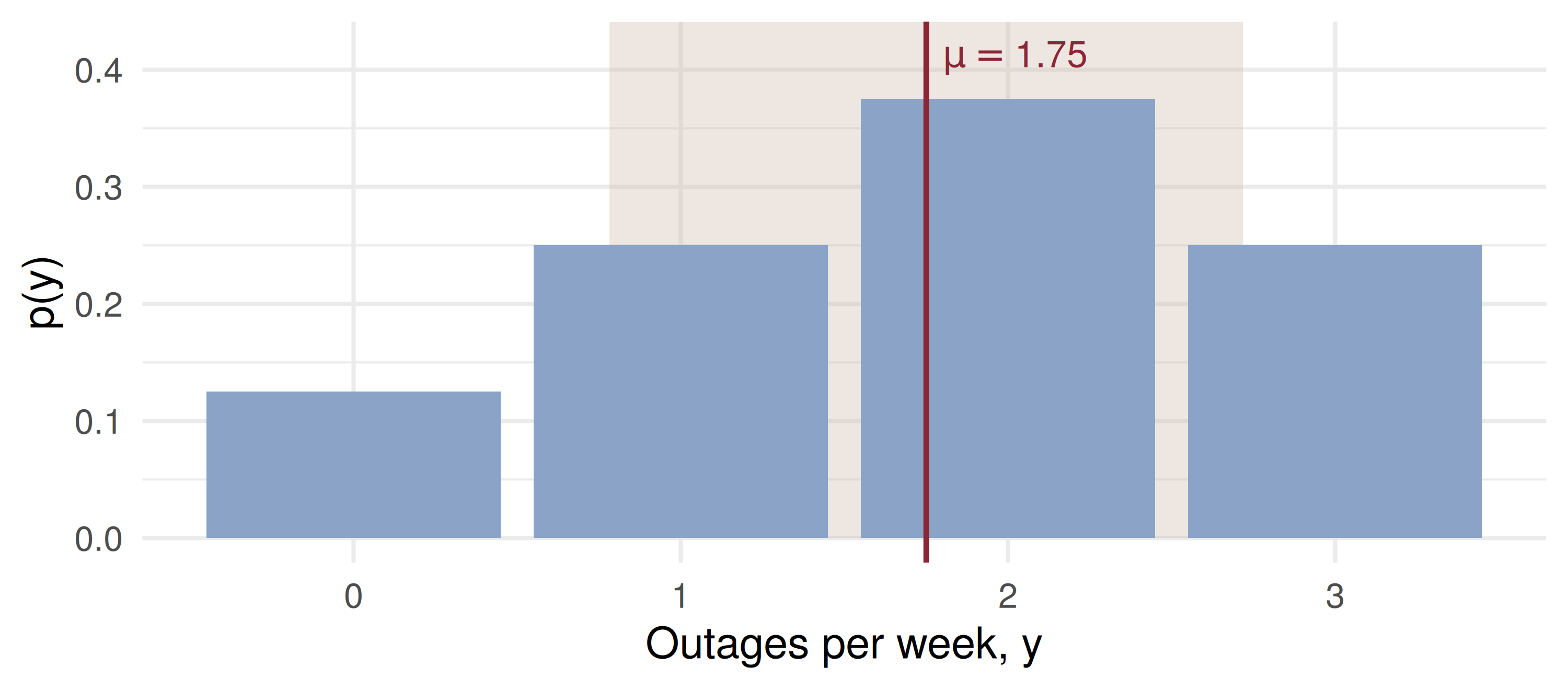
\(Y\) = outages per week on an ISP’s business network in Baku.

\(y\)	0	1	2	3
\(p(y)\)	\(1/8\)	\(1/4\)	\(3/8\)	\(1/4\)

\[\mu = 0\left(\tfrac18\right) + 1\left(\tfrac14\right) + 2\left(\tfrac38\right) + 3\left(\tfrac14\right) = 1.75\]

\[\sigma^2 = (0-1.75)^2\tfrac18 + (1-1.75)^2\tfrac14 + (2-1.75)^2\tfrac38 + (3-1.75)^2\tfrac14 = 0.9375\] \(\sigma = \sqrt{0.9375} = 0.97\). The interval \(\mu \pm \sigma = (0.78, 2.72)\) holds \(y = 1, 2\): probability \(5/8\).

💻 The Same Numbers in R

y <- 0:3
p <- c(1, 2, 3, 2) / 8

mu     <- sum(y * p)                 # Definition 3.4
sigma2 <- sum((y - mu)^2 * p)        # Definition 3.5
round(c(total = sum(p), mu = mu, var = sigma2, sd = sqrt(sigma2)), 4)

 total     mu    var     sd 
1.0000 1.7500 0.9375 0.9682 

# A long run of simulated weeks: the average settles on mu
weeks <- sample(y, 100000, replace = TRUE, prob = p)
round(c(avg = mean(weeks), var = mean((weeks - mean(weeks))^2)), 4)

   avg    var 
1.7475 0.9430 

📈 The Probability Histogram

\(\mu\) sits between bars, at a value \(Y\) can never take. The shaded band is \(\mu \pm \sigma\).

📐 Theorem 3.2: \(E[g(Y)]\)

Theorem 3.2

\(E[g(Y)] = \sum_{\text{all } y} g(y)\,p(y)\)

The ISP’s contract credits a corporate client 0 AZN for 0 or 1 outages, 500 AZN for 2 and 1,500 AZN for 3. \[E[g(Y)] = 0\left(\tfrac18\right) + 0\left(\tfrac14\right) + 500\left(\tfrac38\right) + 1500\left(\tfrac14\right) = 562.5 \text{ AZN per week}\]

No need to derive the distribution of \(g(Y)\) first. The proof does exactly that grouping — \(P(g = 0) = 3/8\), \(P(g = 500) = 3/8\), \(P(g = 1500) = 1/4\) — and gets the same sum.

📐 Theorems 3.3–3.5: Linearity

Theorems 3.3, 3.4 and 3.5

For a constant \(c\) and functions \(g, g_1, \dots, g_k\) of \(Y\): \[E(c) = c, \qquad E[c\,g(Y)] = c\,E[g(Y)],\] \[E[g_1(Y) + \cdots + g_k(Y)] = E[g_1(Y)] + \cdots + E[g_k(Y)]\]

Each proof is one line: apply Theorem 3.2, then pull the constant or split the sum. \(E(c) = c\) uses \(\sum_y p(y) = 1\) from Theorem 3.1.

📐 Theorem 3.6: A Shortcut

Theorem 3.6

\(V(Y) = \sigma^2 = E[(Y - \mu)^2] = E(Y^2) - \mu^2\)

Expand and use 3.3–3.5: \(E(Y^2 - 2\mu Y + \mu^2) = E(Y^2) - 2\mu^2 + \mu^2\).

Example 3.3, ISP outages: \(E(Y^2) = 0 + 1\left(\tfrac14\right) + 4\left(\tfrac38\right) + 9\left(\tfrac14\right) = 4\), so \[\sigma^2 = 4 - 1.75^2 = 0.9375\] Note \(E(Y^2) = 4 \ne \mu^2 = 3.0625\): the mean of a function is not the function of the mean.

💸 A Remittance Fee, \(aY + b\)

A Baku transfer office charges 1 AZN plus 2% of the amount. With \(Y\) = amount in hundreds of AZN, the fee is \(F = 2Y + 1\).

\(y\)	1	2	3	5
\(p(y)\)	0.4	0.3	0.2	0.1

\(E(Y) = 2.1\), \(E(Y^2) = 5.9\), so \(V(Y) = 5.9 - 2.1^2 = 1.49\).

From Theorems 3.3–3.6: \(E(aY + b) = a\mu + b\) and \(V(aY + b) = a^2\sigma^2\). \[E(F) = 2(2.1) + 1 = 5.2 \text{ AZN}, \qquad V(F) = 4(1.49) = 5.96, \quad \sigma_F = 2.44 \text{ AZN}\] The fixed 1 AZN moves the mean and leaves the spread alone.

🌨️ Worked Example: Pricing Hail Cover

One car’s hail claim \(X\) in a season: 0 (prob. 0.95), 2,000 AZN (0.04), 8,000 AZN (0.01). Admin costs 40 AZN per policy; the insurer targets an expected profit of 60 AZN. What premium \(C\)?

\(E(X) = 2000(0.04) + 8000(0.01) = 160\) AZN. Profit is \(C - 40 - X\), so by linearity \[E(\text{profit}) = C - 40 - 160 = 60 \;\Rightarrow\; C = 260 \text{ AZN}\]

\(E(X^2) = 0.04(2000^2) + 0.01(8000^2) = 800{,}000\), so \(\sigma_X = \sqrt{800{,}000 - 160^2} = 880\) AZN — more than three premiums. One policy is a gamble; the business is in pooling many.

🚚 Example 3.4: Two Van Models

A logistics firm runs a van \(t\) hours a day. Daily breakdowns \(Y_A\) have mean and variance \(0.10t\); \(Y_B\) has \(0.12t\). Daily cost (AZN): \(C_A = 10t + 30Y_A^2\), \(C_B = 8t + 30Y_B^2\).

The key step is Theorem 3.6 read backwards, \(E(Y^2) = V(Y) + \mu^2\): \[E(C_A) = 10t + 30[0.10t + (0.10t)^2] = 13t + 0.3t^2, \quad E(C_B) = 11.6t + 0.432t^2\]

\(t\)	\(E(C_A)\)	\(E(C_B)\)	cheaper
10 h	160.0	159.2	B
20 h	380.0	404.8	A

The two cross at \(t = 1.4/0.132 \approx 10.6\) hours.

🧠 Think-Pair-Share

A bank can finance one of two projects. NPV in millions of AZN:

Project	Outcome 1	Outcome 2	Outcome 3
P	\(-1\) (prob. 0.2)	\(2\) (prob. 0.5)	\(4\) (prob. 0.3)
Q	\(1\) (prob. 0.25)	\(2\) (prob. 0.5)	\(3\) (prob. 0.25)

Four minutes, in pairs:

1. Find \(E(Y)\) for each project.
2. Find \(V(Y)\) for each, using Theorem 3.6.
3. Which would a lender who fears losses choose, and what does the mean alone hide?

✅ Think-Pair-Share: Solution

1. \(E(P) = -0.2 + 1.0 + 1.2 = 2.0\) and \(E(Q) = 0.25 + 1.0 + 0.75 = 2.0\). Same mean.

2. \(E(P^2) = 0.2 + 2.0 + 4.8 = 7.0\), so \(V(P) = 7.0 - 4 = 3.0\), \(\sigma_P = 1.73\). \(E(Q^2) = 0.25 + 2.0 + 2.25 = 4.5\), so \(V(Q) = 0.5\), \(\sigma_Q = 0.71\).

3. The mean cannot tell them apart. P carries a 20% chance of losing 1 million; Q never loses. The variance is the first number that sees the difference — which is why §1.3 paired every mean with a spread.

🔬 Interactive: Moving Mass to the Tail

viewof shift = {
  const input = Inputs.range([0, 0.30], {value: 0, step: 0.01,
    label: "Mass moved from 1 to 5 complaints:"});
  ['pointerdown','touchstart','mousedown','click','wheel','pointermove','touchmove']
    .forEach(e => input.addEventListener(e, ev => ev.stopPropagation()));
  return input;
}

base = [0.15, 0.35, 0.25, 0.15, 0.05, 0.05]
pmf = base.map((b, y) => ({y: y, p: y === 1 ? b - shift : y === 5 ? b + shift : b}))
mu = d3.sum(pmf, d => d.y * d.p)
ey2 = d3.sum(pmf, d => d.y * d.y * d.p)
v = ey2 - mu * mu

md`Total **${d3.sum(pmf, d => d.p).toFixed(2)}** · mean **μ = ${mu.toFixed(2)}** · variance **σ² = ${v.toFixed(3)}** · σ = ${Math.sqrt(v).toFixed(3)}`

Plot.plot({
  width: 1150,
  height: 300,
  marginTop: 40,
  marginLeft: 78,
  marginBottom: 58,
  style: {fontSize: "18px"},
  x: {label: "Complaints per hour, y", domain: [0, 1, 2, 3, 4, 5], padding: 0.15},
  y: {label: "p(y)", domain: [0, 0.4], ticks: [0, 0.1, 0.2, 0.3, 0.4], tickFormat: ".1f", grid: true},
  marks: [
    Plot.barY(pmf, {x: "y", y: "p", fill: d => d.y === 1 || d.y === 5 ? "#8b2635" : "#8ba3c7"}),
    Plot.text(pmf, {x: "y", y: "p", text: d => d.p.toFixed(2), dy: -14, fontSize: 18}),
    Plot.ruleY([0])
  ]
})

Moving 0.30 of mass four steps raises μ by \(4(0.30) = 1.2\) — but nearly doubles σ².

📝 Quiz #1: Is It a Distribution?

Which of these can be the probability function of complaints per hour, \(y = 0, 1, 2, 3\)?

• \(p(y) = 0.3, 0.3, 0.3, 0.3\)
• \(p(y) = 0.1, 0.4, 0.3, 0.2\)
• \(p(y) = 0.5, 0.4, 0.2, -0.1\)
• \(p(y) = 0.2, 0.2, 0.2, 0.3\)

📝 Quiz #2: The Mean

A small fleet files \(Y\) = 0, 1 or 2 hail claims in a season, with probabilities 0.5, 0.3, 0.2. What is \(E(Y)\)?

• \(1\), the middle value
• \(0.7\)
• \(0.33\), the average probability
• \(1.1\)

📝 Quiz #3: A Fee Rule

\(V(Y) = 4\) for a transfer amount \(Y\). The fee is \(F = 3Y + 5\) AZN. What is \(V(F)\)?

• \(17\)
• \(12\)
• \(36\)
• \(41\)

📋 Key Formulas

	Statement
Theorem 3.1	\(0 \le p(y) \le 1\), \(\;\sum_y p(y) = 1\)
Definition 3.4	\(E(Y) = \sum_y y\,p(y)\)
Theorem 3.2	\(E[g(Y)] = \sum_y g(y)\,p(y)\)
Definition 3.5	\(V(Y) = E[(Y - \mu)^2]\), \(\;\sigma = \sqrt{V(Y)}\)
Theorems 3.3–3.5	\(E(c) = c\), \(\;E[cg(Y)] = cE[g(Y)]\), \(\;E\) of a sum is the sum of \(E\)
Theorem 3.6	\(V(Y) = E(Y^2) - \mu^2\)
consequence	\(E(aY + b) = a\mu + b\), \(\;V(aY + b) = a^2\sigma^2\)

📋 Summary

• A discrete random variable takes countably many values; its distribution is \(p(y)\) as a formula, a table or a graph

• Theorem 3.1 is the validity check: every \(p(y)\) in \([0, 1]\), total 1

• \(E(Y)\) is a probability-weighted average — a premium is built on it

• \(V(Y)\) measures what the mean hides: two projects with the same mean can carry very different risk

• Linearity and \(E(Y^2) - \mu^2\) turn most calculations into two sums

📚 Practice Problems

Wackerly, 7th edition

• Exercises at the end of §3.2: 3.1, 3.2, 3.9
• Exercises at the end of §3.3: 3.12, 3.13, 3.14, 3.19, 3.23, 3.27, 3.30

Week 5, Problem Set 2 opens today and closes 17 October at 23:59 on WeBWorK, covering §§3.1–3.3. The TA-led tutorial runs this week.

Quiz I is on 17 October, first 30 minutes of class, on Chapters 1–2 — today’s material is not on it, but it is on Midterm I (24 October).

Next class: §3.4 — the binomial distribution.

🙏 Thank You

Dr. Samir Orujov

📧 sorujov@ada.edu.az
🏢 Building D, Room D325
🕓 Office hours: Wednesday, 16:00 – 18:00

Slides and readings: sorujov.net/teaching

❓ Questions

• Can \(E(Y)\) be a value that \(Y\) never takes? Can \(V(Y)\) ever be negative?

• A premium is set at \(E(X)\) plus costs. Why does an insurer with 50 policies charge more than one with 50,000?

• When is \(E[g(Y)] = g(E(Y))\) exactly true?