Mathematical Statistics

🎯 Learning Objectives

By the end of this lecture, you will be able to:

Check an experiment against the five properties of a binomial experiment (Definition 3.6)
Derive \(p(y) = \binom{n}{y} p^y q^{n-y}\) from sample points and the counting rule
Compute binomial probabilities by hand, from Table 1 and with dbinom / pbinom
Use \(E(Y) = np\) and \(V(Y) = npq\) (Theorem 3.7) to price and to judge risk
Read an unlikely count as evidence against an assumed \(p\)

🗺️ Where We Are

Last class ended on: §3.4 — the binomial distribution.

On Wednesday every \(p(y)\) came as a table, and \(E(Y)\) and \(V(Y)\) were two sums over it. Today one formula covers a whole family of tables — indexed by just two numbers, \(n\) and \(p\).

The question this lecture answers

A Baku bank’s SME desk holds 20 loans. Each defaults this year with probability 0.05, independently of the others. How likely are three or more defaults — and how many should the desk budget for?

📐 The Binomial Experiment

Definition 3.6

The experiment consists of a fixed number, \(n\), of identical trials.
Each trial results in one of two outcomes: success, \(S\), or failure, \(F\).
The probability of success on a single trial is equal to some value \(p\) and remains the same from trial to trial. The probability of a failure is \(q = 1 - p\).
The trials are independent.
The random variable of interest is \(Y\), the number of successes observed during the \(n\) trials.

“Success” is only a name for one of the two outcomes. For a credit analyst, a default is the success.

💳 Checking the Five: Card Declines

A payment processor watches the next 8 card transactions at a Baku supermarket. Each is declined with probability \(0.03\), independently. \(Y\) = number declined. Binomial?

Fixed \(n\): 8 transactions, decided in advance. ✔
Two outcomes: declined (\(S\)) or approved (\(F\)). ✔
Same \(p\): \(P(S) = 0.03\) on every transaction. ✔
Independent: stated. ✔
Counts successes: \(Y\) counts declines. ✔ So \(n = 8\), \(p = 0.03\).

“Transactions until the first decline” breaks property 1 — that is §3.5.

🌐 Approximately Binomial

An ISP has 250,000 households in Baku; 35% of them reach the advertised 100 Mbps at peak hour. We test 10 households at random. \(Y\) = number reaching 100 Mbps.

Sampling is without replacement, so strictly the trials are dependent. But removing a few households barely changes the 35%: the conditional probabilities stay very close to \(0.35\), and \(Y\) is approximately binomial with \(n = 10\), \(p = 0.35\).

If the sample were a large fraction of the population — say 10% — this fails, and the right model is the hypergeometric of §3.7.

🧮 Deriving \(p(y)\)

A sample point is an \(n\)-tuple of letters, e.g. \(SSFSF\cdots FS\). Take the one with \(y\) successes first, then \(n - y\) failures: \[S\,S \cdots S\;F\,F \cdots F \quad\text{has probability}\quad (p \cdot p \cdots p)(q \cdot q \cdots q) = p^y q^{n-y}\] by independence (Theorem 2.5, applied \(n\) times): \(y\) factors of \(p\), \(n - y\) factors of \(q\).

Every other ordering of \(y\) \(S\)’s and \(n - y\) \(F\)’s has the same probability, and by Theorem 2.3 there are \(\binom{n}{y} = \frac{n!}{y!(n-y)!}\) of them.

So \(P(Y = y) = \binom{n}{y} p^y q^{n-y}\) — a count times a probability.

📐 Definition 3.7

Definition 3.7

A random variable \(Y\) has a binomial distribution based on \(n\) trials with success probability \(p\) if and only if \[p(y) = \binom{n}{y} p^y q^{n-y}, \qquad y = 0, 1, 2, \dots, n \text{ and } 0 \le p \le 1.\]

Theorem 3.1 holds: each term is positive, and they are the terms of the binomial expansion, \[\sum_{y=0}^{n} \binom{n}{y} p^y q^{n-y} = (q + p)^n = 1^n = 1.\]

🏦 Example: The SME Loan Book

\(n = 20\) loans, default (\(S\)) probability \(p = 0.05\), so \(q = 0.95\).

No defaults: \(\;p(0) = \binom{20}{0}(0.05)^0(0.95)^{20} = 0.3585\)

At least one (the complement, as in Lecture 6): \(\;1 - p(0) = 0.6415\)

Three or more: \(\;P(Y \ge 3) = 1 - [p(0) + p(1) + p(2)]\) \[= 1 - [0.3585 + 0.3774 + 0.1887] = 1 - 0.9245 = 0.0755\] (Terms rounded; the unrounded sum is 0.92452.) With 50,000 AZN per loan, a year of 150,000 AZN or more in defaulted principal has about a 7.5% chance.

💻 The Same Numbers in R

n <- 20; p <- 0.05

round(dbinom(0:4, size = n, prob = p), 4)   # p(0), ..., p(4)

[1] 0.3585 0.3774 0.1887 0.0596 0.0133

c(none         = dbinom(0, n, p),
  at_least_one = 1 - dbinom(0, n, p),
  three_plus   = 1 - pbinom(2, n, p),        # P(Y >= 3) = 1 - P(Y <= 2)
  total        = sum(dbinom(0:n, n, p))) |> round(4)

        none at_least_one   three_plus        total 
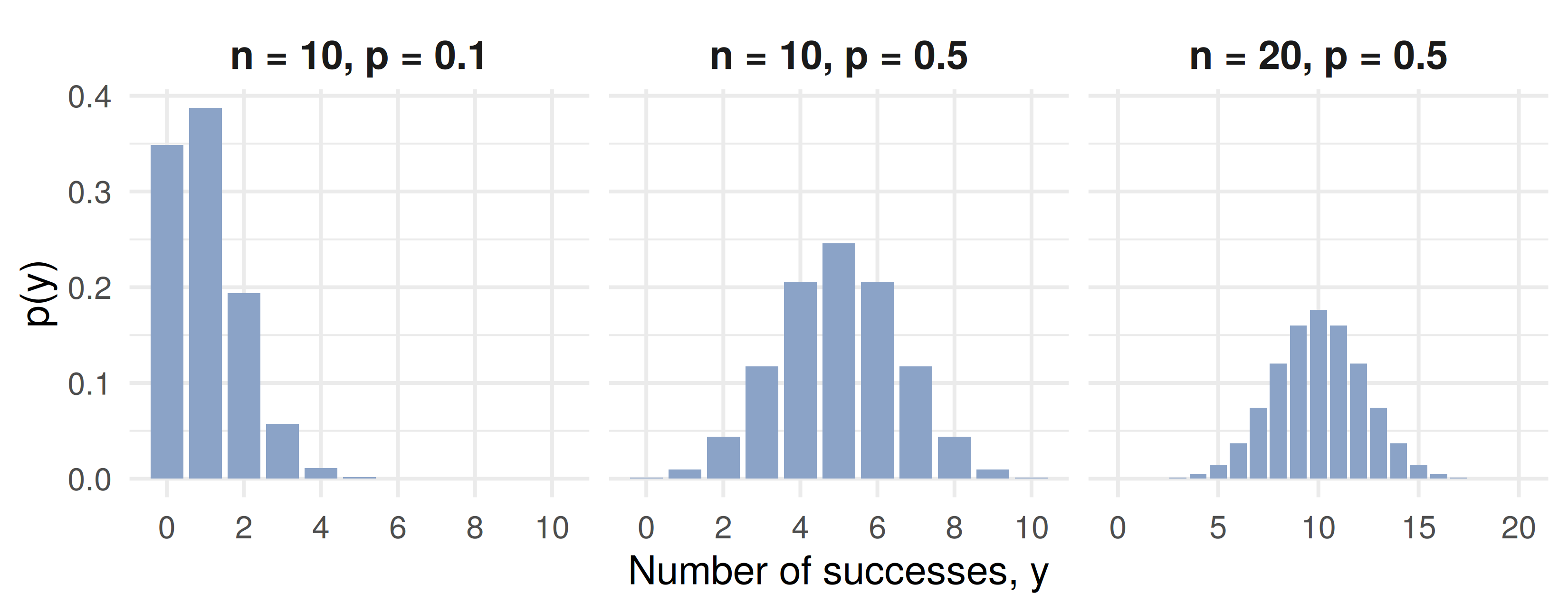
      0.3585       0.6415       0.0755       1.0000

# Simulate 100,000 years of the loan book
years <- rbinom(100000, size = n, prob = p)
round(mean(years >= 3), 4)

[1] 0.0761

📈 The Shape Depends on \(p\) and \(n\)

Small \(p\): piled up near 0 and skewed right. \(p = 0.5\): symmetric. Larger \(n\): wider and lower.

📋 Table 1 and `pbinom`: Card Declines

The acquiring bank’s contract says a terminal’s decline rate is 5%. An auditor pulls \(n = 25\) transactions and finds 4 declines. How surprising is that, if the contract is right?

\[P(Y \ge 4) = 1 - P(Y \le 3) = 1 - \sum_{y=0}^{3} p(y)\] Table 1, Appendix 3: the table for \(n = 25\), column \(p = .05\), row \(a = 3\) gives \(0.966\).

In R: pbinom(3, 25, 0.05) returns the same \(0.966\).

\[P(Y \ge 4) = 1 - 0.966 = 0.034\] Either a 3-in-100 event happened, or the true decline rate is higher than 5%. As in Example 3.9, the auditor has grounds to question the reported rate.

📐 Theorem 3.7: Mean and Variance

Theorem 3.7

Let \(Y\) be a binomial random variable based on \(n\) trials and success probability \(p\). Then \[\mu = E(Y) = np \qquad\text{and}\qquad \sigma^2 = V(Y) = npq.\]

SME book: \(\mu = 20(0.05) = 1\) default a year, \(\sigma^2 = 20(0.05)(0.95) = 0.95\), \(\sigma = 0.975\).

The mean is what intuition says: 5% of 20. The variance is the new information — and \(pq\) is largest at \(p = 0.5\), where the outcome is least predictable.

🔍 The Proof: Two Tricks Worth Keeping

Mean. The \(y = 0\) term vanishes; cancel \(y\) against \(y!\), factor out \(np\), set \(z = y - 1\): \[E(Y) = np \sum_{z=0}^{n-1} \binom{n-1}{z} p^z q^{n-1-z} = np \cdot 1\] The sum is a binomial distribution on \(n - 1\) trials, so it equals 1.

Variance. \(E(Y^2)\) does not cancel against \(y!\), but \(E[Y(Y-1)]\) does. The same device gives \(E[Y(Y-1)] = n(n-1)p^2\), so \[\sigma^2 = E[Y(Y-1)] + \mu - \mu^2 = n(n-1)p^2 + np - n^2p^2 = npq.\]

Trick 1: \(\sum p(y) = 1\) evaluates a sum for free. Trick 2: find \(E[Y(Y-1)]\), not \(E(Y^2)\).

📞 Worked Example: A Sales Shift

A mobile operator’s outbound team makes \(n = 40\) calls a shift; each converts to a sale with \(p = 0.15\), independently. An agent earns 30 AZN base plus 12 AZN per sale.

Sales: \(E(Y) = 40(0.15) = 6\), \(\;V(Y) = 40(0.15)(0.85) = 5.1\), \(\;\sigma = 2.26\).

Pay \(W = 30 + 12Y\) — Wednesday’s linear rule, Theorems 3.3–3.5 and \(V(aY + b) = a^2 V(Y)\): \[E(W) = 30 + 12(6) = 102 \text{ AZN}, \qquad V(W) = 12^2(5.1) = 734.4, \qquad \sigma_W = 27.10 \text{ AZN}\]

A 10-sale shift (150 AZN): \(P(Y \ge 10) = 1 -\) pbinom(9, 40, 0.15) \(= 0.067\).

🎯 Using the Model Backwards

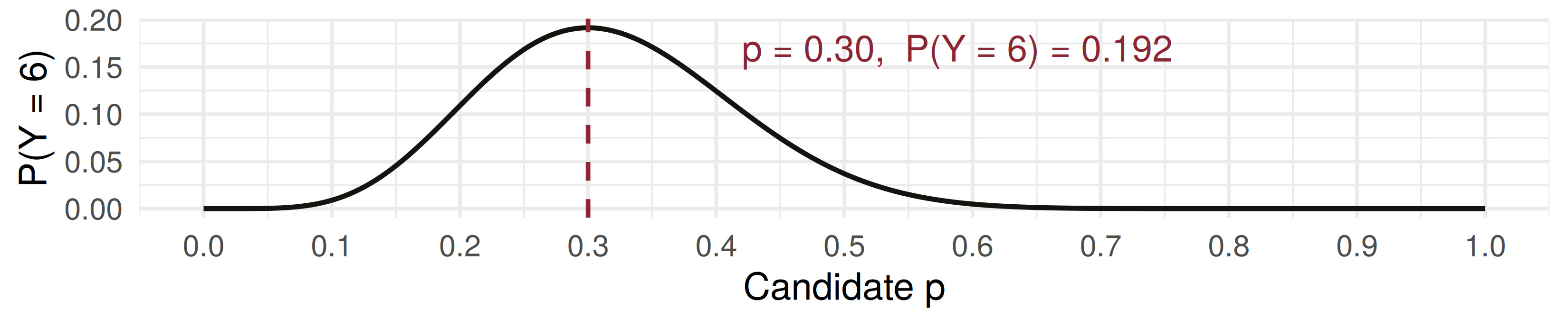
The regulator tests 20 households of a new ISP and 6 reach 100 Mbps. Which \(p\) makes that result most probable? (Example 3.10)

Maximise \(\ln P(Y = 6) = \ln\binom{20}{6} + 6\ln p + 14\ln(1-p)\): \[\frac{6}{p} - \frac{14}{1-p} = 0 \;\Rightarrow\; \hat{p} = \frac{6}{20} = 0.30\]

🧠 Think-Pair-Share

A microfinance lender in Ganja holds 10 independent loans of 8,000 AZN each. Each defaults with probability 0.10, and a default loses the full principal.

Four minutes, in pairs:

What is the probability that no loan defaults?
What is the probability of two or more defaults?
What are the mean and standard deviation of the AZN loss?

✅ Think-Pair-Share: Solution

\(Y \sim\) binomial with \(n = 10\), \(p = 0.10\), \(q = 0.90\).

\(p(0) = (0.9)^{10} = 0.3487\)
\(p(1) = \binom{10}{1}(0.1)(0.9)^9 = 0.3874\), so \(P(Y \ge 2) = 1 - 0.3487 - 0.3874 = 0.2639\)

Loss \(L = 8000\,Y\). \(E(Y) = np = 1\) and \(V(Y) = npq = 0.9\), so \[E(L) = 8{,}000 \text{ AZN}, \qquad \sigma_L = 8000\sqrt{0.9} = 7{,}589 \text{ AZN}\] The standard deviation is nearly as large as the mean: ten loans are too few to diversify away default risk.

🔬 Interactive: How \(p\) Moves the Shape

Code

viewof p_hit = {
  const input = Inputs.range([0.05, 0.95], {value: 0.35, step: 0.01,
    label: "p, each household hits 100 Mbps:"});
  ['pointerdown','touchstart','mousedown','click','wheel','pointermove','touchmove']
    .forEach(e => input.addEventListener(e, ev => ev.stopPropagation()));
  return input;
}

Code

Plot.plot({
  width: 1150,
  height: 300,
  marginTop: 40,
  marginLeft: 78,
  marginBottom: 58,
  style: {fontSize: "18px"},
  x: {label: "Households of 20 reaching 100 Mbps, y", domain: d3.range(0, 21), padding: 0.15},
  y: {label: "p(y)", domain: [0, 0.4], ticks: [0, 0.1, 0.2, 0.3, 0.4], tickFormat: ".1f", grid: true},
  marks: [
    Plot.barY(pmfB, {x: "y", y: "p",
      fill: d => d.y === Math.round(nTest * p_hit) ? "#8b2635" : "#8ba3c7"}),
    Plot.ruleY([0])
  ]
})

The red bar is the one nearest \(np\). Near \(p = 0.05\) or \(0.95\) the mass piles against an end; at \(p = 0.5\) it is symmetric and widest.

📝 Quiz #1: Is It Binomial?

Which of these random variables has a binomial distribution?

The number of 50 card transactions declined, each declined with probability 0.03, independently
The number of cold calls made until the first sale
The total AZN value of 20 independent transactions
The number of bad loans in a file review of 6 drawn from a pool of 10 loans, 3 of them bad

📝 Quiz #2: The Variance

A telecom sells to each of \(n = 50\) contacted customers with probability \(p = 0.2\), independently. What is \(V(Y)\)?

\(8\)
\(10\)
\(2.83\)
\(40\)

📝 Quiz #3: Which Outcome Is the Success?

Each of 8 independent SME loans defaults with probability 0.1. \(Y\) = number of loans that repay. What is \(P(Y = 8)\)?

\(0.9^8 = 0.4305\)
\(0.1^8 = 10^{-8}\)
\(1 - 0.9^8 = 0.5695\)
\(8 \times 0.9 = 7.2\)

📋 Key Formulas

	Statement
Definition 3.7	\(p(y) = \binom{n}{y} p^y q^{n-y}, \quad y = 0, 1, \dots, n\)
validity	\(\sum_{y=0}^{n} p(y) = (q + p)^n = 1\)
at least one	\(P(Y \ge 1) = 1 - q^n\)
Theorem 3.7	\(E(Y) = np, \qquad V(Y) = npq\)
\(p(y)\) in R	`dbinom(y, n, p)`
\(P(Y \le a)\) in R	`pbinom(a, n, p)`
estimate of \(p\) (Ex. 3.10)	\(\hat{p} = y/n\)

📋 Summary

A binomial experiment: fixed \(n\), two outcomes, constant \(p\), independent trials, \(Y\) counts successes
Sampling a small part of a large population is approximately binomial; a large part is not (§3.7)
\(p(y)\) is a count, \(\binom{n}{y}\), times the probability of one ordering, \(p^y q^{n-y}\)
\(E(Y) = np\) and \(V(Y) = npq\); with Wednesday’s linear rules they price a loss or a pay scheme
An improbable count under an assumed \(p\) is evidence against that \(p\)
Name the success first — then make sure \(p\) is its probability

📚 Practice Problems

Wackerly, 7th edition, exercises at the end of §3.4:

3.38, 3.39, 3.40, 3.43, 3.48, 3.54, 3.56, 3.57, 3.59

Week 6, Problem Set 1 is open now and closes Sunday 25 October at 23:59 on WeBWorK, covering §3.4.

Quiz I is this Saturday, 17 October, in the first 30 minutes of class, on Chapters 1–2.

Next class: Saturday 17 October — the geometric and negative binomial distributions, Wackerly §§3.5–3.6: what happens when the number of trials is the random quantity.

🙏 Thank You

Dr. Samir Orujov

📧 sorujov@ada.edu.az
🏢 Building D, Room D325
🕓 Office hours: Wednesday, 16:00 – 18:00

Slides and readings: sorujov.net/teaching

❓ Questions

Loan defaults tend to rise together in a recession. Which property of Definition 3.6 does that break, and in which direction does it push \(P(Y \ge 3)\)?
If \(Y\) is binomial\((n, p)\), what is the distribution of \(n - Y\)?
For fixed \(n\), which \(p\) makes \(V(Y)\) largest, and why is that the hardest book to reserve for?

Mathematical Statistics

🎯 Learning Objectives

🗺️ Where We Are

📐 The Binomial Experiment

💳 Checking the Five: Card Declines

🌐 Approximately Binomial

🧮 Deriving \(p(y)\)

📐 Definition 3.7

🏦 Example: The SME Loan Book

💻 The Same Numbers in R

📈 The Shape Depends on \(p\) and \(n\)

📋 Table 1 and pbinom: Card Declines

📐 Theorem 3.7: Mean and Variance

🔍 The Proof: Two Tricks Worth Keeping

📞 Worked Example: A Sales Shift

🎯 Using the Model Backwards

🧠 Think-Pair-Share

✅ Think-Pair-Share: Solution

🔬 Interactive: How \(p\) Moves the Shape

📝 Quiz #1: Is It Binomial?

📝 Quiz #2: The Variance

📝 Quiz #3: Which Outcome Is the Success?

📋 Key Formulas

📋 Summary

📚 Practice Problems

🙏 Thank You

❓ Questions

📋 Table 1 and `pbinom`: Card Declines