Mathematical Statistics

The Hypergeometric and Poisson Distributions; Midterm I Review

Samir Orujov, PhD

ADA University, School of Business

Information Communication Technologies Agency, Statistics Unit

2026-09-24

🎯 Learning Objectives

By the end of this lecture, you will be able to:

• Recognise sampling without replacement from a finite pool, and model it with the hypergeometric distribution

• Compute hypergeometric probabilities, mean and variance, and explain the factor \(\frac{N-n}{N-1}\)

• Apply the Poisson distribution to counts of events in time, including a Poisson process over \(a\) units

• Use the Poisson as the limit of the binomial for rare events

• Choose among the five discrete models of Chapter 3 for Midterm I

🗺️ Where We Are

Wackerly §3.7–3.8

Saturday ended on one sentence: the binomial fixes the trials; the geometric and negative binomial fix the successes and count the trials. All three rest on the same two assumptions — independent trials with a constant \(p\).

Today we drop the assumptions themselves, one at a time. Draw without replacement from a small pool and independence fails: that is the hypergeometric. Let \(n \to \infty\) while \(p \to 0\) and there is no \(n\) left to count: that is the Poisson.

🧾 Why the Binomial Fails in an Audit

An auditor receives a batch of 25 invoices from a Baku construction supplier. Unknown to her, 5 are misstated. She pulls 6 at random for testing.

The first draw is misstated with probability \(5/25 = 0.20\). If it was, the second is misstated with probability \(4/24 = 0.167\); if it was not, \(5/24 = 0.208\).

The trials are not independent and \(p\) is not constant, so \(Y\), the number of misstated invoices in the sample, is not binomial. It is a counting problem over subsets — Section 2.6 — and that is where the book derives the answer.

📐 Definition 3.10: Hypergeometric

Definition 3.10

A random variable \(Y\) has a hypergeometric probability distribution if and only if \[p(y) = \frac{\binom{r}{y}\binom{N-r}{n-y}}{\binom{N}{n}},\] where \(y\) is an integer \(0, 1, 2, \ldots, n\), subject to \(y \le r\) and \(n - y \le N - r\).

Numerator: choose \(y\) of the \(r\) “red” elements and \(n-y\) of the \(N-r\) others (the \(mn\) rule). Denominator: all \(\binom{N}{n}\) equally likely samples. In R: dhyper(y, r, N - r, n).

📊 Worked Example: The Audit Rule

The firm’s rule: escalate to a full audit if two or more of the 6 sampled invoices are misstated. With \(N = 25\), \(r = 5\), \(n = 6\):

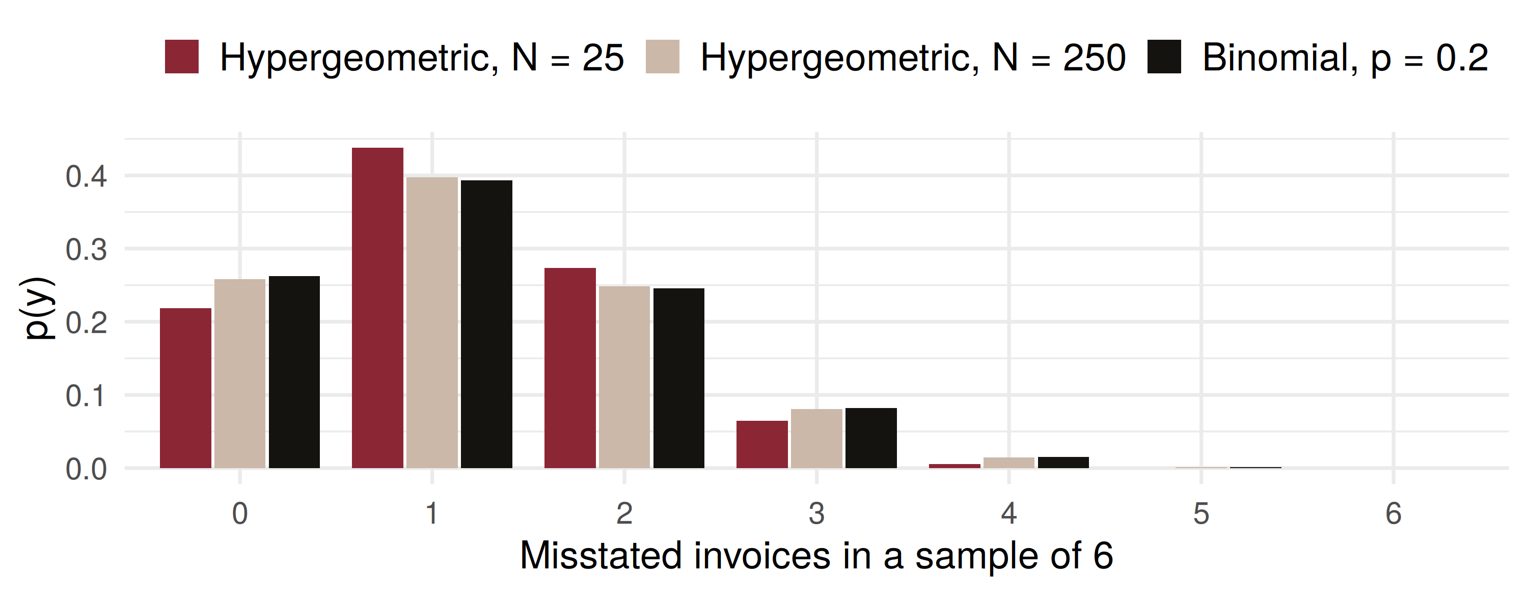
\[p(0) = \frac{\binom{5}{0}\binom{20}{6}}{\binom{25}{6}} = \frac{38760}{177100} = 0.2189, \qquad p(1) = \frac{\binom{5}{1}\binom{20}{5}}{\binom{25}{6}} = \frac{77520}{177100} = 0.4377\]

\[P(Y \ge 2) = 1 - p(0) - p(1) = 1 - 0.2189 - 0.4377 = 0.3434\]

A batch with one invoice in five misstated still passes the test about two times in three. The complement did the work, exactly as in Chapter 2.

📐 Theorem 3.10: Mean and Variance

Theorem 3.10

If \(Y\) has a hypergeometric distribution, \[\mu = E(Y) = \frac{nr}{N} \qquad \sigma^2 = V(Y) = n\left(\frac{r}{N}\right)\left(\frac{N-r}{N}\right)\left(\frac{N-n}{N-1}\right)\]

With \(p = r/N\) this is \(\mu = np\) and \(\sigma^2 = npq\,\frac{N-n}{N-1}\): the binomial, times a finite-population correction.

Audit: \(\mu = 6(5)/25 = 1.2\) and \(\sigma^2 = 6(0.2)(0.8)(19/24) = 0.76\). The binomial would say \(0.96\) — sampling without replacement removes about a fifth of the variance.

💻 When Does the Pool Size Matter?

Same \(r/N = 0.2\) throughout. At \(N = 250\) the sample is 2.4% of the pool and the hypergeometric is indistinguishable from the binomial; at \(N = 25\) it is 24% and the distribution is visibly tighter.

🌧️ From Binomial to Poisson

Split a day into \(n\) tiny subintervals, each holding at most one event with probability \(p\), independently. The count is binomial. Now let \(n \to \infty\) with \(\lambda = np\) fixed: \[\lim_{n\to\infty}\binom{n}{y}p^y(1-p)^{n-y} = \frac{\lambda^y}{y!}e^{-\lambda}\]

Definition 3.11

\(Y\) has a Poisson probability distribution if and only if \[p(y) = \frac{\lambda^y}{y!}e^{-\lambda}, \qquad y = 0, 1, 2, \ldots, \quad \lambda > 0.\]

📦 Worked Example: A Claims Desk

The cargo-insurance desk of a Baku insurer receives on average \(\lambda = 3\) claims per day, and can fully process 4 in a day. Let \(Y\) be tomorrow’s claim count.

\[P(Y = 0) = e^{-3} = 0.0498 \quad P(Y = 1) = 3e^{-3} = 0.1494 \quad P(Y = 2) = 4.5e^{-3} = 0.2240\]

The desk falls behind when \(Y \ge 5\): \[P(Y \ge 5) = 1 - P(Y \le 4) = 1 - 0.8153 = 0.1847\]

Roughly one working day in five leaves a backlog. In R: 1 - ppois(4, 3), or Table 3 of Appendix 3.

📐 Theorem 3.11: Mean = Variance

Theorem 3.11

If \(Y\) has a Poisson distribution with parameter \(\lambda\), then \(\mu = E(Y) = \lambda\) and \(\sigma^2 = V(Y) = \lambda\).

Proof idea. In \(\sum_{y} y\,\lambda^y e^{-\lambda}/y!\) the \(y = 0\) term vanishes; cancel \(y\) against \(y!\), factor out \(\lambda\), and put \(z = y - 1\). What remains is a Poisson sum, which equals 1. The variance is Exercise 3.138.

A practical test: if claim counts show a sample variance far above their mean, the Poisson model — not just its \(\lambda\) — is in doubt.

🏧 A Poisson Process: One ATM

If events occur as a Poisson process at \(\lambda\) per unit, the count in \(a\) units is Poisson with mean \(a\lambda\). An ATM in Nizami Street averages 12 withdrawals per hour.

lambda_hr <- 12
hours <- c(1/6, 1/2, 1, 2)
data.frame(
  window     = c("10 min", "30 min", "1 hour", "2 hours"),
  mean       = hours * lambda_hr,
  P_none     = round(exp(-hours * lambda_hr), 4),
  P_over_30  = round(1 - ppois(30, hours * lambda_hr), 4))

   window mean P_none P_over_30
1  10 min    2 0.1353    0.0000
2  30 min    6 0.0025    0.0000
3  1 hour   12 0.0000    0.0000
4 2 hours   24 0.0000    0.0958

No withdrawal in 10 minutes: \(e^{-2} = 0.1353\). A cassette good for 30 withdrawals runs out within 2 hours with probability \(0.0958\).

⚠️ The Poisson Limit: Rare Losses

A bank’s trading desk has a loss event (a failed settlement, a fat-finger trade) on any of 250 trading days with probability 0.008, independently. Binomial, or Poisson with \(\lambda = np = 2\)?

y <- 0:5
data.frame(y,
  binomial = round(dbinom(y, 250, 0.008), 4),
  poisson  = round(dpois(y, 2), 4))

  y binomial poisson
1 0   0.1343  0.1353
2 1   0.2707  0.2707
3 2   0.2718  0.2707
4 3   0.1812  0.1804
5 4   0.0902  0.0902
6 5   0.0358  0.0361

Agreement to the third decimal: \(P(Y \ge 4)\) is \(0.1421\) exact and \(0.1429\) Poisson. The book’s rule of thumb: large \(n\), small \(p\), \(\lambda = np\) below about 7.

🔬 Interactive: Binomial to Poisson

viewof n_sub = {
  const input = Inputs.range([4, 200], {value: 6, step: 1,
    label: "Number of trials n (λ = np = 2):"});
  ['pointerdown','touchstart','mousedown','click','wheel','pointermove','touchmove']
    .forEach(e => input.addEventListener(e, ev => ev.stopPropagation()));
  return input;
}

lam = 2
binomPmf = (n, p) => {
  const out = [Math.pow(1 - p, n)];
  for (let k = 0; k < 10; k++) out.push(k + 1 > n ? 0 : out[k] * (n - k) / (k + 1) * p / (1 - p));
  return out;
}
poisPmf = Array.from({length: 11}, (_, k) => {
  let f = 1; for (let i = 2; i <= k; i++) f *= i;
  return Math.exp(-lam) * Math.pow(lam, k) / f;
})
bin = binomPmf(n_sub, lam / n_sub).map((p, k) => ({y: k, p}))
pois = poisPmf.map((p, k) => ({y: k, p}))
gap = d3.max(bin, (d, k) => Math.abs(d.p - pois[k].p))

md`With **n = ${n_sub}** and **p = ${(lam / n_sub).toFixed(4)}**, the largest gap between binomial bars and Poisson dots is **${gap.toFixed(4)}**.`

Plot.plot({
  width: 1150,
  height: 300,
  marginLeft: 78,
  marginBottom: 58,
  style: {fontSize: "18px"},
  x: {label: "y", domain: d3.range(0, 11), padding: 0.25},
  y: {label: "p(y)", domain: [0, 0.45], tickFormat: ".2f"},
  marks: [
    Plot.barY(bin, {x: "y", y: "p", fill: "#cbb8a9"}),
    Plot.dot(pois, {x: "y", y: "p", r: 8, fill: "#8b2635"}),
    Plot.ruleY([0])
  ]
})

🧠 Think-Pair-Share

A bank’s risk desk has recorded operational-loss events as a Poisson process at 2 per month for years. Last quarter (3 months) there were 11.

Four minutes, in pairs:

1. What is the distribution of \(Y\), the number of events in a quarter?

2. Where does 11 fall relative to \(\mu \pm 2\sigma\)?

3. Is 11 alarming enough to report to the risk committee?

✅ Think-Pair-Share: Solution

1. A Poisson process over \(a = 3\) months: \(Y\) is Poisson with \(\lambda^\star = 3 \times 2 = 6\).

2. Theorem 3.11: \(\mu = 6\), \(\sigma = \sqrt{6} = 2.45\), so \(\mu + 2\sigma = 6 + 2(2.45) = 10.90\). The observed 11 lies just outside.

3. Exactly: \(P(Y \ge 11) = 1 - P(Y \le 10) = 1 - 0.9574 = 0.0426\), from 1 - ppois(10, 6).

Not impossible, but a one-in-25 quarter under the old rate — worth an investigation into whether \(\lambda\) has risen, which is the reasoning of Example 3.22.

📝 Quiz #1: A Licence Lottery

The Energy Ministry awards 6 solar licences by lottery among 16 bidders, of whom 4 are joint ventures. What is the probability that no joint venture wins?

• \(\binom{12}{6}\big/\binom{16}{6} = 0.1154\)
• \((0.75)^6 = 0.1780\)
• \(\binom{12}{6}\big/\binom{16}{4} = 0.5077\)
• \(12/16 = 0.75\)

📝 Quiz #2: Scaling the Interval

Withdrawals at an ATM follow a Poisson process at 12 per hour. What is the probability of no withdrawal in a 5-minute window?

• \(e^{-1} = 0.368\)
• \(e^{-12} = 0.000006\)
• \(1 - e^{-1} = 0.632\)
• \(1/12 = 0.083\)

🧭 Review: Which Discrete Model?

Model	\(Y\) is…	\(E(Y)\)	\(V(Y)\)
Binomial §3.4	successes in \(n\) independent trials	\(np\)	\(npq\)
Geometric §3.5	the trial of the first success	\(1/p\)	\(q/p^2\)
Negative binomial §3.6	the trial of the \(r\)-th success	\(r/p\)	\(rq/p^2\)
Hypergeometric §3.7	“red” items in \(n\) drawn without replacement	\(nr/N\)	\(npq\frac{N-n}{N-1}\)
Poisson §3.8	events in a fixed interval	\(\lambda\)	\(\lambda\)

Ask in order: is \(n\) fixed? Independent trials, binomial; a finite pool, hypergeometric. Is the trial count the variable? Geometric or negative binomial. Only a rate? Poisson.

✍️ Exam-Style Question 1

Of a bank’s 12 branches, 3 failed an internal compliance check. The Central Bank inspects 4 branches chosen at random. Find the probability that it finds at least one failing branch, and the mean and variance of the number it finds.

Without replacement from \(N = 12\) with \(r = 3\), \(n = 4\): \[P(Y \ge 1) = 1 - \frac{\binom{3}{0}\binom{9}{4}}{\binom{12}{4}} = 1 - \frac{126}{495} = 0.7455\]

\(\mu = 4(3)/12 = 1\) and \(\sigma^2 = 4(0.25)(0.75)(8/11) = 0.5455\). Treating it as binomial would give \(1 - 0.75^4 = 0.6836\) — wrong, and by 6 points.

✍️ Exam-Style Question 2

Large claims (above 50,000 AZN) reach a reinsurer as a Poisson process at 0.5 per week. Call a 4-week month quiet if it has at most one large claim. Months are independent. Find the probability that at least 2 of the next 6 months are quiet.

Step 1 (§3.8). A month has \(\lambda = 4(0.5) = 2\): \(w = P(Y \le 1) = e^{-2} + 2e^{-2} = 3e^{-2} = 0.4060\).

Step 2 (§3.4). Quiet months \(X\) are binomial with \(n = 6\), \(p = w = 0.4060\): \[P(X \ge 2) = 1 - (0.5940)^6 - 6(0.4060)(0.5940)^5 = 1 - 0.0439 - 0.1801 = 0.7759\]

📝 Quiz #3: Exam-Style — A Cost Built on a Count

Claims at a desk are Poisson with \(\lambda = 4\) per day. Daily handling cost is \(C = 500 + 800Y\) AZN. What is the standard deviation of \(C\)?

• \(1600\) AZN
• \(3200\) AZN
• \(3700\) AZN
• \(2100\) AZN

📋 Key Formulas

	Statement
Definition 3.10	\(p(y) = \binom{r}{y}\binom{N-r}{n-y}\big/\binom{N}{n}\)
Theorem 3.10	\(\mu = \frac{nr}{N}\), \(\ \sigma^2 = n\frac{r}{N}\frac{N-r}{N}\frac{N-n}{N-1}\)
Definition 3.11	\(p(y) = \frac{\lambda^y}{y!}e^{-\lambda}\), \(\ y = 0, 1, 2, \ldots\)
Theorem 3.11	\(\mu = \sigma^2 = \lambda\)
Poisson process	count in \(a\) units is Poisson with mean \(a\lambda\)
Poisson limit	\(\binom{n}{y}p^y q^{n-y} \approx \frac{(np)^y}{y!}e^{-np}\), large \(n\), small \(p\)

📋 Summary

• Drawing without replacement from a small pool breaks independence: the count is hypergeometric

• Its mean is the binomial’s \(np\); its variance is \(npq\) shrunk by \(\frac{N-n}{N-1}\), which matters when \(n/N\) is not small

• Counts of rare events in an interval are Poisson, and the single parameter \(\lambda\) is both the mean and the variance

• Over \(a\) units of a Poisson process the mean is \(a\lambda\); for large \(n\) and small \(p\) the binomial is close to Poisson(\(np\))

• For Midterm I, name the model before computing: fixed \(n\)? finite pool? trials to a success? only a rate?

📚 Practice Problems

Wackerly, 7th edition

• §3.7: Exercises 3.103, 3.105, 3.108, 3.112, 3.117
• §3.8: Exercises 3.121, 3.122, 3.126, 3.128, 3.134, 3.139

Week 7, Problem Set 1 is open now and closes Sunday 1 November at 23:59 on WeBWorK, covering §§3.7–3.8. It is the only set this week.

Midterm Examination I is on Saturday 24 October: Chapters 1–3, §§3.1–3.8.

Next class: 28 October, after the midterm — moments and moment-generating functions (Wackerly §3.9).

🙏 Thank You

Dr. Samir Orujov

📧 sorujov@ada.edu.az
🏢 Building D, Room D325
🕓 Office hours: Wednesday, 16:00 – 18:00

Slides and readings: sorujov.net/teaching

❓ Questions

• In the audit, how large must the batch \(N\) be before the binomial answer is within 0.005 of the hypergeometric one?

• Why can a Poisson count exceed any bound, when a binomial count never exceeds \(n\)?

• Two independent ATMs average 12 and 8 withdrawals an hour. What would you guess the distribution of their total is — and how would you check it?