Mathematical Statistics

Moments and Moment-Generating Functions

Samir Orujov, PhD

ADA University, School of Business

Information Communication Technologies Agency, Statistics Unit

2026-09-24

🎯 Learning Objectives

By the end of this lecture, you will be able to:

• Distinguish moments about the origin \(\mu^{\text{ʹ}}_k\) from central moments \(\mu_k\)

• Derive the moment-generating function of a Poisson or binomial count

• Recover \(E(Y)\) and \(V(Y)\) from \(m(t)\) by differentiating at \(t = 0\) (Theorem 3.12)

• Transform an MGF when a count becomes a P&L: \(m_{aY+b}(t) = e^{bt}m_Y(at)\)

• Identify a distribution from its MGF, using uniqueness

🗺️ Where We Are

Wackerly §3.9 · first lecture after Midterm I

On 21 October we met the last two discrete models of the chapter, the hypergeometric and the Poisson, and then reviewed §§3.1–3.8 for Saturday’s midterm.

For every model so far, \(\mu\) and \(\sigma^2\) cost a new series trick: the binomial theorem, a geometric sum, \(E[Y(Y-1)]\) for the Poisson.

Today: one function per distribution that hands over every moment by differentiation — and, more importantly, names the distribution.

❓ Motivating Question

A Baku bank’s treasury counts large (\(\geq\) 1M AZN) corporate payments cleared per hour at two branches.

Payments \(y\)	0	1	2	3	4
Branch A, \(p(y)\)	0	1/2	0	1/2	0
Branch B, \(p(y)\)	1/8	0	3/4	0	1/8

Both have \(\mu = 2\) and \(\sigma^2 = 1\).

The question

If two counts share a mean and a variance, is the risk the same? And what extra numbers would pin the distribution down?

📐 Definitions 3.12 and 3.13

Definition 3.12

The \(k\)th moment of \(Y\) taken about the origin is \(E(Y^k)\), denoted \(\mu^{\text{ʹ}}_k\).

Definition 3.13

The \(k\)th moment of \(Y\) taken about its mean, the \(k\)th central moment, is \(E[(Y-\mu)^k]\), denoted \(\mu_k\).

So \(\mu^{\text{ʹ}}_1 = \mu\), \(\mu_2 = \sigma^2\), and Theorem 3.6 reads \(\sigma^2 = \mu^{\text{ʹ}}_2 - (\mu^{\text{ʹ}}_1)^2\).

💻 Two Branches, Four Moments

yA <- c(1, 3);    pA <- c(1/2, 1/2)
yB <- c(0, 2, 4); pB <- c(1/8, 3/4, 1/8)
mom <- function(y, p, k, about = 0) sum((y - about)^k * p)

data.frame(k = 1:4,
  A_origin  = sapply(1:4, \(k) mom(yA, pA, k)),
  B_origin  = sapply(1:4, \(k) mom(yB, pB, k)),
  A_central = sapply(1:4, \(k) mom(yA, pA, k, 2)),
  B_central = sapply(1:4, \(k) mom(yB, pB, k, 2)))

  k A_origin B_origin A_central B_central
1 1        2        2         0         0
2 2        5        5         1         1
3 3       14       14         0         0
4 4       41       44         1         4

Identical up to \(k = 3\); the fourth moment separates them. Branch B has more mass far from the mean — fatter tails.

📐 Definition 3.14: The MGF

Definition 3.14

The moment-generating function \(m(t)\) for a random variable \(Y\) is \(m(t) = E(e^{tY})\). We say that an MGF for \(Y\) exists if there is a constant \(b > 0\) such that \(m(t)\) is finite for \(|t| \leq b\).

For a discrete \(Y\) it is one sum: \[m(t) = \sum_y e^{ty}p(y)\] It is a function of \(t\), not of \(y\); the \(y\)’s have been summed out. And always \(m(0) = \sum_y p(y) = 1\).

🔑 Why “Moment-Generating”?

Expand \(e^{ty} = 1 + ty + \dfrac{(ty)^2}{2!} + \dfrac{(ty)^3}{3!} + \cdots\) and take expectations term by term:

\[m(t) = 1 + t\mu^{\text{ʹ}}_1 + \frac{t^2}{2!}\mu^{\text{ʹ}}_2 + \frac{t^3}{3!}\mu^{\text{ʹ}}_3 + \cdots\]

\(\mu^{\text{ʹ}}_k\) is the coefficient of \(t^k/k!\). The MGF is every moment of \(Y\) packed into one expression.

Swapping the sum over \(y\) with the infinite series is justified whenever \(m(t)\) exists near 0.

📐 Theorem 3.12

Theorem 3.12

If \(m(t)\) exists, then for any positive integer \(k\), \[\left.\frac{d^k m(t)}{dt^k}\right|_{t=0} = m^{(k)}(0) = \mu^{\text{ʹ}}_k\]

Differentiate the series \(k\) times: every term below \(t^k\) vanishes, the \(t^k\) term leaves \(\mu^{\text{ʹ}}_k\), and every higher term still carries a power of \(t\), so it dies at \(t = 0\).

In practice: \(\mu = m^{\text{ʹ}}(0)\) and \(\sigma^2 = m^{\text{ʹʹ}}(0) - [m^{\text{ʹ}}(0)]^2\).

🚗 Example 3.23: Motor Claims

A Baku motor insurer’s daily claim count is \(Y \sim\) Poisson(\(\lambda\)).

\[m(t) = \sum_{y=0}^{\infty} e^{ty}\frac{\lambda^y e^{-\lambda}}{y!} = e^{-\lambda}\sum_{y=0}^{\infty}\frac{(\lambda e^t)^y}{y!}\]

The sum is the Taylor series of \(e^{\lambda e^t}\), so \[m(t) = e^{-\lambda}e^{\lambda e^t} = e^{\lambda(e^t - 1)}\]

The same trick as in Theorem 3.11: turn what is left into a Poisson p.f. with mean \(\lambda e^t\), which sums to 1.

🧮 Example 3.24: Mean and Variance

\[m^{\text{ʹ}}(t) = e^{\lambda(e^t-1)}\,\lambda e^t, \qquad m^{\text{ʹʹ}}(t) = e^{\lambda(e^t-1)}(\lambda e^t)^2 + e^{\lambda(e^t-1)}\lambda e^t\]

At \(t = 0\): \(\mu = m^{\text{ʹ}}(0) = \lambda\) and \(\mu^{\text{ʹ}}_2 = m^{\text{ʹʹ}}(0) = \lambda^2 + \lambda\), so \[\sigma^2 = \lambda^2 + \lambda - \lambda^2 = \lambda\]

With \(\lambda = 4.5\) claims a day: \(\mu^{\text{ʹ}}_2 = 24.75\), \(\sigma^2 = 4.5\), \(\sigma = 2.12\). No \(E[Y(Y-1)]\) detour needed.

📈 The Binomial MGF: Winning Trades

An FX dealer books \(n = 10\) independent trades a day, each profitable with \(p = 0.6\). \(Y\) = winning trades \(\sim\) Bin\((10, 0.6)\). By the binomial theorem (Exercise 3.145): \[m(t) = \sum_{y=0}^{n}\binom{n}{y}(pe^t)^y q^{n-y} = (pe^t + q)^n\]

\(m^{\text{ʹ}}(0) = np = 6\), and \(m^{\text{ʹʹ}}(0) = n(n-1)p^2 + np = 32.4 + 6 = 38.4\), so \[V(Y) = 38.4 - 6^2 = 2.4 = npq\]

💰 From Trade Count to Daily P&L

Each winner earns 2 thousand AZN, each loser costs 1: \(X = 2Y - (10 - Y) = 3Y - 10\).

Exercise 3.156

If \(X = aY + b\), then \(m_X(t) = E(e^{t(aY+b)}) = e^{bt}\,m_Y(at)\).

\[m_X(t) = e^{-10t}\,(0.6e^{3t} + 0.4)^{10}\] Differentiating at 0: \(E(X) = 3(6) - 10 = 8\) thousand AZN, \(V(X) = 9(2.4) = 21.6\), \(\sigma_X = 4.65\).

💻 Checking Theorem 3.12 Numerically

mgf <- function(t, y, p) sapply(t, \(s) sum(exp(s * y) * p))
h <- 1e-4
d1 <- function(m) (m(h) - m(-h)) / (2 * h)            # m'(0)
d2 <- function(m) (m(h) - 2 * m(0) + m(-h)) / h^2     # m''(0)

claims <- \(t) mgf(t, 0:200, dpois(0:200, 4.5))
x <- 3 * (0:10) - 10                                   # P&L support
pnl    <- \(t) mgf(t, x, dbinom(0:10, 10, 0.6))

round(rbind(claims = c(mean = d1(claims), var = d2(claims) - d1(claims)^2),
            pnl    = c(mean = d1(pnl),    var = d2(pnl)    - d1(pnl)^2)), 3)

       mean  var
claims  4.5  4.5
pnl     8.0 21.6

Brute-force sums and finite differences agree with the calculus: 4.5 and 4.5, 8 and 21.6.

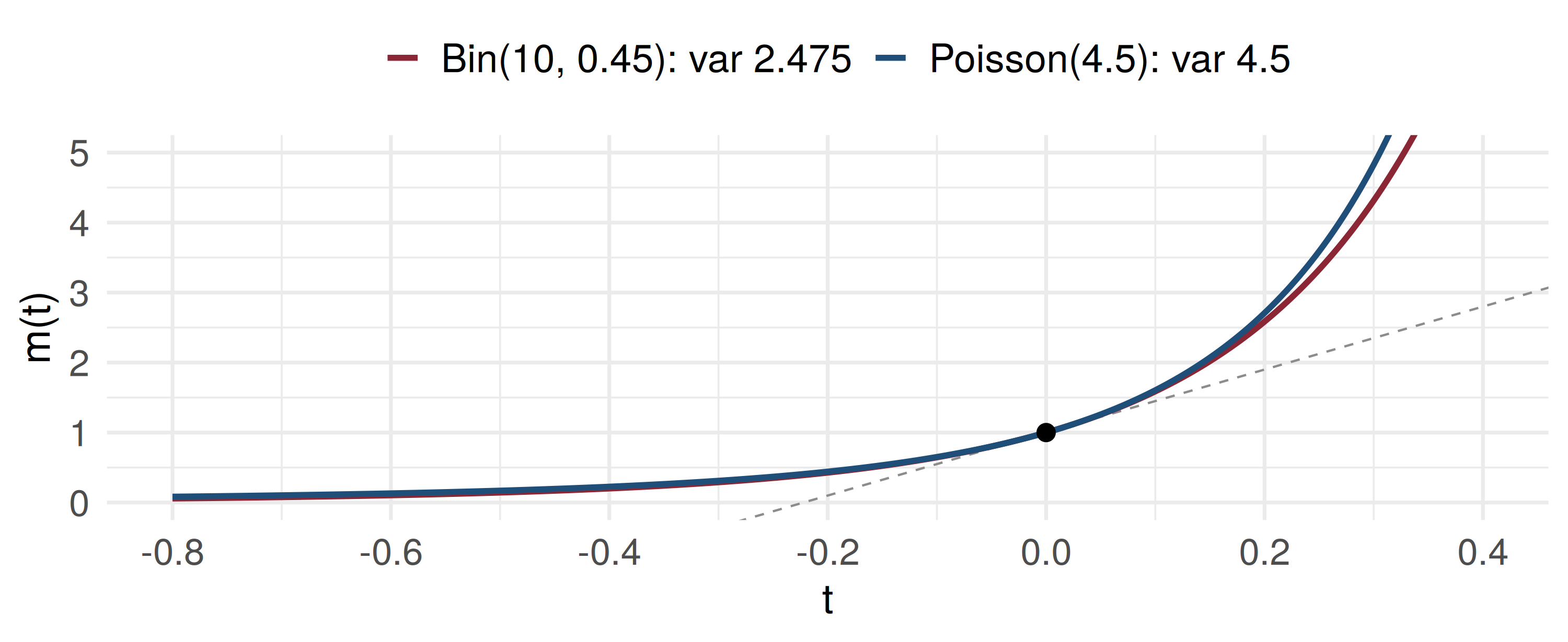
🖼️ Same Slope, Different Curvature

Slope at 0 is the mean, curvature is \(E(Y^2)\). Both counts average 4.5, so both curves leave \((0, 1)\) along the dashed tangent. The Poisson bends up faster: \(\mu^{\text{ʹ}}_2 = 24.75\) against \(22.725\).

🔐 The Primary Use: Uniqueness

If \(m(t)\) exists for \(p(y)\), it is unique. If \(m_Y(t) = m_Z(t)\) for all \(|t| < b\), some \(b > 0\), then \(Y\) and \(Z\) have the same distribution.

Example 3.25, re-set. A bank’s monthly count of operational-loss events has \(m_Y(t) = e^{3.2(e^t - 1)}\).

That is the Poisson MGF with \(\lambda = 3.2\), so \(Y \sim\) Poisson(3.2): mean and variance 3.2, and a loss-free month has probability \(e^{-3.2} = 0.0408\).

🧭 A Recognition Table

Distribution	\(m(t)\)	Source
Binomial\((n, p)\)	\((pe^t + q)^n\)	Exercise 3.145
Geometric\((p)\)	\(\dfrac{pe^t}{1 - qe^t}\)	Exercise 3.147
Poisson\((\lambda)\)	\(e^{\lambda(e^t - 1)}\)	Example 3.23

Of 12 SME loan applications, \(Y\) approved has \(m(t) = (0.3e^t + 0.7)^{12}\). So \(Y \sim\) Bin(12, 0.3): \(\mu = 3.6\), \(\sigma^2 = 2.52\), \(P(Y = 0) = 0.7^{12} = 0.0138\).

🧠 Think-Pair-Share

A mobile operator’s count of regional network outages per day has \[m(t) = 0.5 + 0.3e^{t} + 0.2e^{2t}\]

Four minutes, in pairs:

1. What is the distribution of \(Y\)? (Read it off: \(m(t) = \sum_y e^{ty}p(y)\).)

2. Find \(E(Y)\) and \(V(Y)\) from \(m(t)\).

3. Check both directly from \(p(y)\).

✅ Think-Pair-Share: Solution

1. Match \(\sum_y e^{ty}p(y)\) term by term: \(p(0) = 0.5\), \(p(1) = 0.3\), \(p(2) = 0.2\). Uniqueness says that is the distribution.

2. \(m^{\text{ʹ}}(t) = 0.3e^t + 0.4e^{2t}\), so \(E(Y) = 0.7\). \(m^{\text{ʹʹ}}(t) = 0.3e^t + 0.8e^{2t}\), so \(E(Y^2) = 1.1\) and \(V(Y) = 1.1 - 0.49 = 0.61\).

3. Directly: \(0(0.5) + 1(0.3) + 2(0.2) = 0.7\) and \(0 + 0.3 + 4(0.2) = 1.1\). Same numbers — the MGF is just a disciplined way to do those sums.

📝 Quiz #1: Variance From an MGF

Daily chargebacks at a card acquirer have \(m(t) = e^{2.5(e^t - 1)}\). What is \(V(Y)\)?

• \(2.5\)
• \(6.25\)
• \(8.75\)
• \(1.58\)

📝 Quiz #2: Name the Distribution

Out of 15 export shipments, \(Y\) are held at customs, with \(m(t) = (0.2e^t + 0.8)^{15}\). What is the distribution of \(Y\)?

• Binomial with \(n = 15\), \(p = 0.2\)
• Binomial with \(n = 15\), \(p = 0.8\)
• Poisson with \(\lambda = 3\)
• Geometric with \(p = 0.2\)

📝 Quiz #3: A Linear Change

\(Y\) has MGF \(m_Y(t)\). A fee schedule charges \(W = 2Y + 3\) AZN. What is \(m_W(t)\)?

• \(e^{3t}\,m_Y(2t)\)
• \(2\,m_Y(t) + 3\)
• \(e^{2t}\,m_Y(3t)\)
• \(m_Y(2t) + 3\)

📋 Key Formulas

	Statement
Defs 3.12, 3.13	\(\mu^{\text{ʹ}}_k = E(Y^k)\), \(\mu_k = E[(Y - \mu)^k]\)
Def 3.14	\(m(t) = E(e^{tY}) = \sum_y e^{ty}p(y)\)
Theorem 3.12	\(m^{(k)}(0) = \mu^{\text{ʹ}}_k\)
mean, variance	\(\mu = m^{\text{ʹ}}(0)\), \(\sigma^2 = m^{\text{ʹʹ}}(0) - [m^{\text{ʹ}}(0)]^2\)
linear change	\(m_{aY+b}(t) = e^{bt}m_Y(at)\)
binomial, Poisson	\((pe^t + q)^n\), \(e^{\lambda(e^t - 1)}\)

📋 Summary

• Mean and variance do not determine a distribution; the full sequence of moments (usually) does

• The MGF packs every moment into one function: \(\mu^{\text{ʹ}}_k\) is the coefficient of \(t^k/k!\)

• Differentiate \(k\) times and set \(t = 0\) to read off \(\mu^{\text{ʹ}}_k\)

• A count turned into a P&L by \(aY + b\) changes its MGF to \(e^{bt}m_Y(at)\)

• Uniqueness is the main use: recognise the MGF, and you know the distribution

📚 Practice Problems

Wackerly, 7th edition

• Exercises at the end of §3.9 — start with 3.145 and 3.146 (the binomial MGF), then 3.149, 3.153 – 3.155

• Exercises 3.156 – 3.157: the linear-change rule, and why a shift leaves the variance alone

Week 8, Problem Set 1 is open now and closes Sunday 8 November at 23:59 on WeBWorK, covering §3.9.

Next class: 31 October — probability-generating functions, Tchebysheff’s theorem, and Chapter 3 in review (Wackerly §3.10–3.11).

🙏 Thank You

Dr. Samir Orujov

📧 sorujov@ada.edu.az
🏢 Building D, Room D325
🕓 Office hours: Wednesday, 16:00 – 18:00

Slides and readings: sorujov.net/teaching

❓ Questions

• Branches A and B agreed on three moments. Can you build two counts that agree on four?

• Why must every MGF satisfy \(m(0) = 1\), and what does that say about the tangent line in today’s figure?

• If \(Y_1\) and \(Y_2\) are independent Poisson claim counts, what might \(m_{Y_1 + Y_2}(t)\) be?