Mathematical Statistics

Continuous Random Variables: Distribution and Density Functions

Samir Orujov, PhD

ADA University, School of Business

Information Communication Technologies Agency, Statistics Unit

2026-09-24

🎯 Learning Objectives

By the end of this lecture, you will be able to:

• Write the distribution function \(F(y) = P(Y \le y)\) of any random variable, discrete or continuous

• Explain why \(P(Y = y) = 0\) for a continuous \(Y\), and what replaces a probability function

• Move between a density \(f(y)\) and its distribution function \(F(y)\) by integrating or differentiating

• Compute \(P(a \le Y \le b)\) as an area under \(f(y)\), and find the constant that makes \(f(y)\) a density

• Find a quantile \(\phi_p\), such as the median settlement time of a payment

🗺️ Where We Are

Wackerly §§4.1–4.2

Friday closed Chapter 3 with a map of the discrete models: name the counting mechanism, pick the model, read off \(E(Y)\) and \(V(Y)\). Every one of them assigned a probability \(p(y)\) to each value.

Today we leave counts behind. The time a payment takes to settle, the share of a credit line a firm draws, a day’s move in the exchange rate: these take any value in an interval.

For those, \(p(y)\) cannot work. Chapter 4 replaces it with two functions, \(F(y)\) and \(f(y)\), and today is about both.

❓ Motivating Question

The payments desk’s problem

A Baku bank sends cross-border transfers that settle anywhere between 0 and 4 hours after release. The desk promises corporate clients settlement within 3 hours.

What is the probability a transfer settles in exactly 2 hours? And in at most 3?

The first question has the surprising answer zero, and yet the second has a perfectly good answer. By the end of today we will compute it: \(27/32 \approx 0.844\).

📐 Definition 4.1 and Theorem 4.1

Definition 4.1

Let \(Y\) denote any random variable. The distribution function of \(Y\), denoted by \(F(y)\), is such that \(F(y) = P(Y \le y)\) for \(-\infty < y < \infty\).

Theorem 4.1: Properties of a Distribution Function

1. \(F(-\infty) \equiv \lim_{y \to -\infty} F(y) = 0\)
2. \(F(\infty) \equiv \lim_{y \to \infty} F(y) = 1\)
3. \(F(y)\) is nondecreasing: if \(y_1 < y_2\) then \(F(y_1) \le F(y_2)\)

Note the word any: \(F(y)\) exists for discrete variables too.

🪜 A Discrete F Is a Staircase

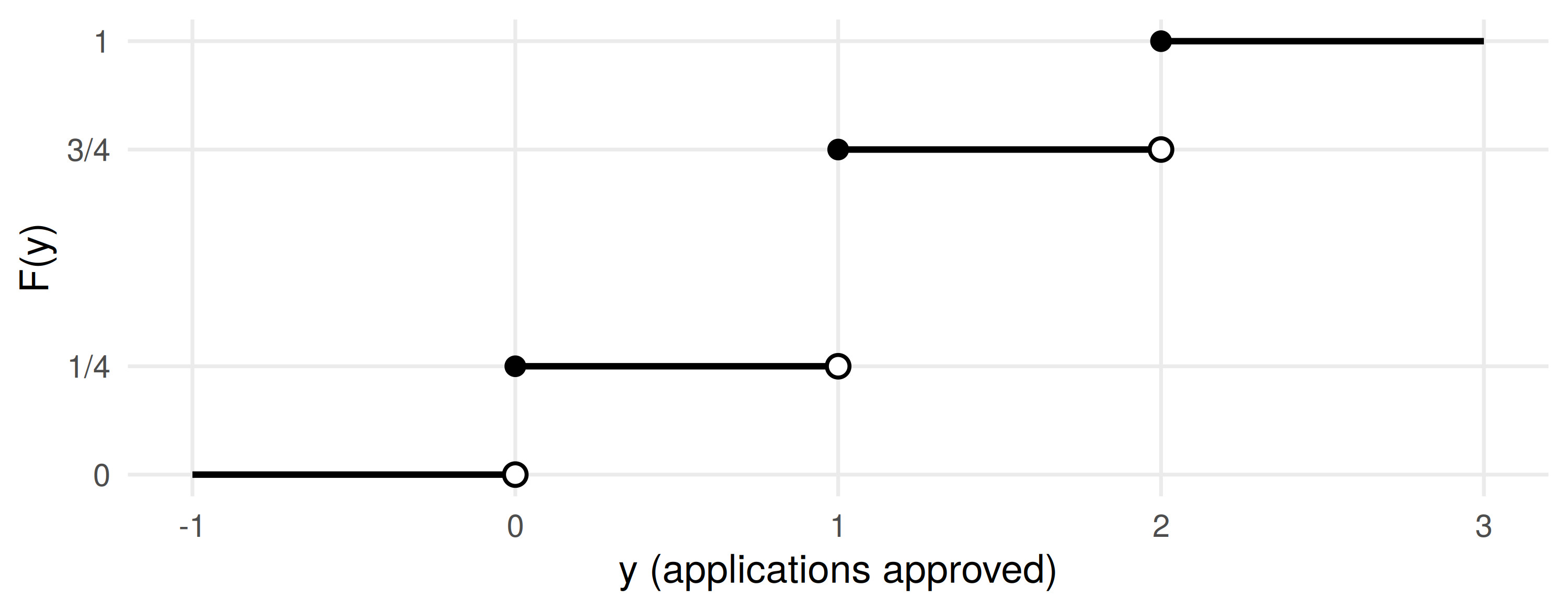
Example 4.1, in a loan office: two SME applications, each approved independently with probability \(1/2\). \(Y\) = number approved, so \(p(0) = 1/4\), \(p(1) = 1/2\), \(p(2) = 1/4\) and, for instance, \(F(1.5) = 1/4 + 1/2 = 3/4\).

📐 Definition 4.2: When F Has No Jumps

The staircase jumps at 0, 1, 2 by exactly \(p(0)\), \(p(1)\), \(p(2)\). It is flat in between because those values carry no probability.

Definition 4.2

A random variable \(Y\) with distribution function \(F(y)\) is said to be continuous if \(F(y)\) is continuous, for \(-\infty < y < \infty\).

Consequence. If \(Y\) is continuous, \(P(Y = y) = 0\) for every real \(y\). A point with \(P(Y = y_0) = p_0 > 0\) would put a jump of size \(p_0\) into \(F\). So a transfer settling in exactly 2.000… hours has probability zero, while one settling between 2 and 3 hours does not.

📐 Definition 4.3: The Density

Definition 4.3

Let \(F(y)\) be the distribution function for a continuous random variable \(Y\). Then \(f(y) = \dfrac{dF(y)}{dy}\), wherever the derivative exists, is called the probability density function for \(Y\). Equivalently, \(F(y) = \int_{-\infty}^{y} f(t)\, dt\).

Theorem 4.2: Properties of a Density Function

1. \(f(y) \ge 0\) for all \(y\), \(-\infty < y < \infty\)
2. \(\int_{-\infty}^{\infty} f(y)\, dy = 1\)

💳 Worked Example: A Credit Line

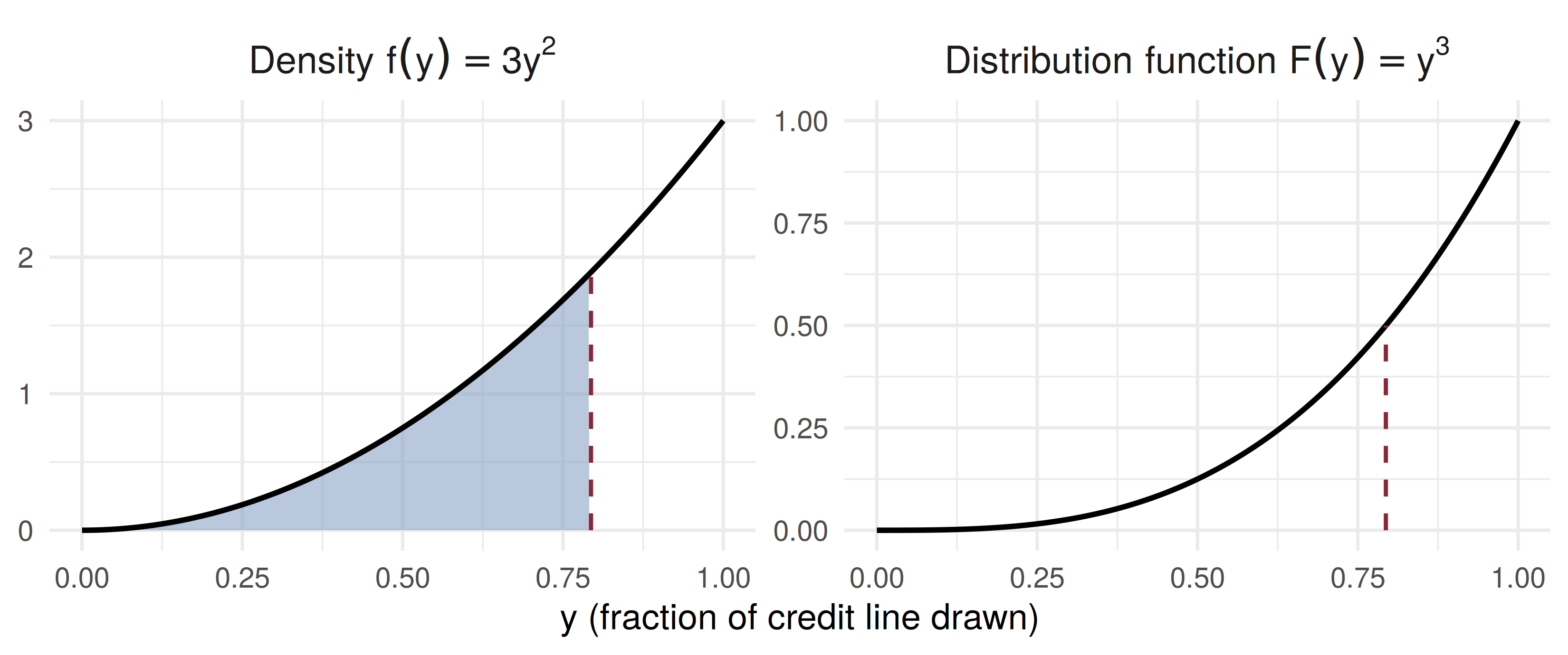
Example 4.3, re-set. \(Y\) is the fraction of its approved credit line a corporate client has drawn at month-end: \[f(y) = \begin{cases} 3y^2, & 0 \le y \le 1, \\ 0, & \text{elsewhere.} \end{cases}\]

Integrate from \(-\infty\) up to \(y\). Below 0 nothing accumulates; above 1 everything already has: \[F(y) = \begin{cases} 0, & y < 0, \\ \int_0^y 3t^2\, dt = y^3, & 0 \le y \le 1, \\ 1, & y > 1. \end{cases}\]

So \(P(Y \le 0.5) = 0.5^3 = 0.125\): only one client in eight uses half the line or less. Clients draw heavily.

📈 f and F Side by Side

The shaded area on the left, 0.5, is the height of \(F\) on the right at the same \(y\). And \(f(1) = 3\): a density may exceed 1; \(F\) never does.

📐 Definition 4.4: Quantiles

Definition 4.4

Let \(Y\) denote any random variable. If \(0 < p < 1\), the \(p\)th quantile of \(Y\), denoted by \(\phi_p\), is the smallest value such that \(F(\phi_p) = P(Y \le \phi_p) \ge p\). If \(Y\) is continuous, \(\phi_p\) is the smallest value such that \(F(\phi_p) = p\).

Credit line: solve \(\phi_p^3 = p\).

• Median: \(\phi_{.5} = 0.5^{1/3} = 0.7937\). On a 500,000 AZN line, half of clients have drawn more than 396,850 AZN.
• \(\phi_{.90} = 0.9^{1/3} = 0.9655\): the bank’s liquidity desk plans for 96.5% utilisation in the top decile.

📐 Theorem 4.3: Probability Is Area

Theorem 4.3

If the random variable \(Y\) has density function \(f(y)\) and \(a < b\), then the probability that \(Y\) falls in the interval \([a, b]\) is \[P(a \le Y \le b) = \int_a^b f(y)\, dy = F(b) - F(a)\]

Because \(P(Y = a) = P(Y = b) = 0\), the endpoints do not matter: \[P(a < Y < b) = P(a \le Y < b) = P(a < Y \le b) = P(a \le Y \le b)\] This is false for discrete variables. In the loan office, \(P(0 < Y < 2) = 1/2\) but \(P(0 \le Y \le 2) = 1\).

🏦 Worked Example: Settlement Time

Examples 4.4–4.5, re-set. Settlement time \(Y\) (hours) has \(f(y) = c\,y(4 - y)\) for \(0 \le y \le 4\), zero elsewhere. Step 1: find \(c\). \[\int_0^4 c(4y - y^2)\, dy = c\left[2y^2 - \frac{y^3}{3}\right]_0^4 = c\left(32 - \frac{64}{3}\right) = \frac{32}{3}c = 1 \;\Rightarrow\; c = \frac{3}{32}\]

Step 2: the distribution function. For \(0 \le y \le 4\), \(F(y) = \dfrac{6y^2 - y^3}{32}\).

Step 3: read off the desk’s answers. \[P(Y \le 3) = \frac{54 - 27}{32} = \frac{27}{32} = 0.8438, \qquad P(1 \le Y \le 3) = \frac{27}{32} - \frac{5}{32} = 0.6875\] The 3-hour promise is broken for about one transfer in six, \(5/32 = 0.156\).

💻 Checking It in R

f <- function(y) ifelse(y >= 0 & y <= 4, y * (4 - y), 0)
c_const <- 1 / integrate(f, 0, 4)$value            # should be 3/32
dens <- function(y) c_const * f(y)
Fy   <- function(y) integrate(dens, 0, y)$value

c(c = c_const, P_le_3 = Fy(3), P_1_to_3 = Fy(3) - Fy(1))

       c   P_le_3 P_1_to_3 
 0.09375  0.84375  0.68750 

# quantiles: solve F(phi) = p numerically
q <- function(p) uniroot(function(y) Fy(y) - p, c(0, 4))$root
round(c(median = q(0.5), phi_90 = q(0.9)), 4)

median phi_90 
2.0000 3.2168 

The median is 2 hours, by symmetry. Nine transfers in ten settle within 3.22 hours.

🔬 Interactive: Area Under f Is the Height of F

viewof b = {
  const input = Inputs.range([0, 4], {value: 3, step: 0.05,
    label: "Settlement deadline b (hours):"});
  ['pointerdown','touchstart','mousedown','click','wheel','pointermove','touchmove']
    .forEach(e => input.addEventListener(e, ev => ev.stopPropagation()));
  return input;
}

dens = y => (3 / 32) * y * (4 - y)
cdf = y => (6 * y * y - y * y * y) / 32
grid = Array.from({length: 161}, (_, i) => ({y: i * 0.025, f: dens(i * 0.025)}))
shaded = grid.filter(d => d.y <= b + 1e-9)

md`Shaded area = F(${b.toFixed(2)}) = P(Y ≤ ${b.toFixed(2)}) = **${cdf(b).toFixed(4)}**`

Plot.plot({
  width: 1150,
  height: 320,
  marginLeft: 78,
  marginBottom: 58,
  style: {fontSize: "18px"},
  x: {label: "Settlement time y (hours)", domain: [0, 4], ticks: [0, 0.5, 1, 1.5, 2, 2.5, 3, 3.5, 4]},
  y: {label: "Density f(y)", domain: [0, 0.4], ticks: [0, 0.1, 0.2, 0.3, 0.4], tickFormat: ".1f"},
  marks: [
    Plot.areaY(shaded, {x: "y", y: "f", fill: "#8ba3c7", fillOpacity: 0.7}),
    Plot.line(grid, {x: "y", y: "f", stroke: "#14130f", strokeWidth: 2.5}),
    Plot.ruleX([b], {stroke: "#8b2635", strokeWidth: 2, strokeDasharray: "5 4"}),
    Plot.ruleY([0])
  ]
})

🏧 From F to f: Service Time at a Branch

Example 4.2 runs the other way: start from \(F\) and differentiate. A branch’s teller service time \(Y\) (minutes) has \[F(y) = 1 - e^{-y^2/50}, \quad y \ge 0 \qquad \Rightarrow \qquad f(y) = \frac{dF(y)}{dy} = \frac{y}{25}\,e^{-y^2/50}, \quad y \ge 0\]

• A customer takes longer than 10 minutes: \(1 - F(10) = e^{-2} = 0.1353\)
• Between 5 and 10 minutes: \(F(10) - F(5) = e^{-0.5} - e^{-2} = 0.4712\)
• Median: \(1 - e^{-y^2/50} = 0.5\) gives \(\phi_{.5} = \sqrt{50 \ln 2} = 5.89\) minutes

No integral was needed: when \(F\) is given, every probability is a subtraction.

🧠 Think-Pair-Share

The daily move \(Y\) (in %) of the EUR/AZN rate is modelled by \[f(y) = 1 - |y|, \quad -1 \le y \le 1, \qquad 0 \text{ elsewhere.}\]

Four minutes, in pairs:

1. Check that \(f\) is a density. (Sketch it first.)

2. Find \(P(|Y| > 0.5)\), the chance of a move of more than half a percent.

3. Find \(\phi_{.95}\). And what is \(P(Y = 0)\), where \(f\) is highest?

✅ Think-Pair-Share: Solution

1. \(f \ge 0\), and the graph is a triangle with base 2 and height 1: area \(= \tfrac{1}{2} \times 2 \times 1 = 1\).

2. Each tail beyond \(\pm 0.5\) is a triangle with base and height \(0.5\), area \(0.125\). So \(P(|Y| > 0.5) = 0.25\).

3. For \(0 \le y \le 1\), \(F(y) = 1 - \tfrac{(1-y)^2}{2}\). Setting \(F(\phi) = 0.95\) gives \((1 - \phi)^2 = 0.1\), so \[\phi_{.95} = 1 - \sqrt{0.1} = 0.6838\%\] A move above 0.68% happens on about one trading day in twenty.

And \(P(Y = 0) = 0\). \(f(0) = 1\) is a height, not a probability; probability lives only in areas.

📝 Quiz #1: Height or Probability?

The settlement density has \(f(2) = 0.375\). What is \(P(Y = 2)\)?

• \(0\)
• \(0.375\)
• \(0.5\), because 2 is the median
• It cannot be found without \(F(y)\)

📝 Quiz #2: Making a Density

A density is \(f(y) = cy\) for \(0 \le y \le 4\) and \(0\) elsewhere. What is \(c\)?

• \(1/4\)
• \(1/8\)
• \(1/16\)
• \(1/2\)

📝 Quiz #3: Reading F

The credit-line fraction has \(F(y) = y^3\) on \([0, 1]\). What is the probability a client has drawn more than half the line?

• \(0.125\)
• \(0.5\)
• \(0.875\)
• \(0.75\)

📋 Key Formulas

	Statement
Definition 4.1	\(F(y) = P(Y \le y)\), for any random variable
Theorem 4.1	\(F(-\infty) = 0\), \(F(\infty) = 1\), \(F\) nondecreasing
continuous \(Y\)	\(P(Y = y) = 0\) for every \(y\)
Definition 4.3	\(f(y) = dF(y)/dy\), \(\;F(y) = \int_{-\infty}^{y} f(t)\,dt\)
Theorem 4.2	\(f(y) \ge 0\), \(\;\int_{-\infty}^{\infty} f(y)\,dy = 1\)
Theorem 4.3	\(P(a \le Y \le b) = \int_a^b f(y)\,dy = F(b) - F(a)\)
Definition 4.4	\(F(\phi_p) = p\), \(Y\) continuous

📋 Summary

• \(F(y) = P(Y \le y)\) describes every random variable; a discrete one has a staircase, a continuous one has none

• For continuous \(Y\), single points carry probability zero, so endpoints never matter

• The density \(f\) is the derivative of \(F\); \(F\) is the accumulated area under \(f\)

• A density is a height, not a probability, and may exceed 1

• Probabilities are areas, \(F(b) - F(a)\); quantiles invert \(F\)

📚 Practice Problems

Wackerly, 7th edition

• §4.2: Exercises 4.1 – 4.19; start with 4.8, 4.11, 4.12 and 4.14

• Exercise 4.7 is the discrete-endpoints warning from Theorem 4.3, worked from the binomial table

• Redo the settlement example with the deadline moved to 2.5 hours: how often is the promise broken?

Week 9, Problem Set 1 is open now and closes Sunday 15 November at 23:59 on WeBWorK, covering §§4.1–4.2.

Next class: 7 November, expected values for continuous random variables, and our first named continuous model, the uniform distribution (Wackerly §§4.3–4.4).

🙏 Thank You

Dr. Samir Orujov

📧 sorujov@ada.edu.az
🏢 Building D, Room D325
🕓 Office hours: Wednesday, 16:00 – 18:00

Slides and readings: sorujov.net/teaching

❓ Questions

• A distribution function can have jumps and rise smoothly in between. What kind of variable would that describe in insurance?

• If \(f(y) = 3y^2\) on \([0,1]\), why is \(f(1) = 3\) not a contradiction of \(P \le 1\)?

• The bank reports the 90th percentile of settlement time rather than the mean. Why might a client prefer that number?