Mathematical Statistics

Independent Random Variables

Samir Orujov, PhD

ADA University, School of Business

Information Communication Technologies Agency, Statistics Unit

2026-09-24

🎯 Learning Objectives

By the end of this lecture, you will be able to:

  • State Definition 5.8: \(Y_1, Y_2\) are independent when \(F(y_1, y_2) = F_1(y_1)F_2(y_2)\)

  • Test a joint table cell by cell with Theorem 5.4, and stop at the first cell that fails

  • Apply the factorisation criterion (Theorem 5.5) to a joint density without finding its marginals

  • Recognise a support that is not a rectangle as a proof of dependence

  • Explain why co-moving asset returns cannot be priced as independent

πŸ—ΊοΈ Where We Are

Wackerly Β§5.4

Saturday (Β§5.3): a marginal removes a variable, \(p_1(y_1) = \sum_{y_2} p(y_1, y_2)\); a conditional keeps one slice of the joint and divides by its total, \(p(y_1 \mid y_2) = p(y_1, y_2)/p_2(y_2)\).

We ended on the question for today: what does it mean when conditioning on one variable leaves the other’s distribution unchanged? Then learning \(Y_2\) tells you nothing about \(Y_1\), and the joint is just the two marginals multiplied.

❓ The Question

Two branches, one cash van

A Baku bank refills the ATMs of two branches, one in Nizami and one in Khatai, from a single cash centre. Does a heavy day of withdrawals in Nizami make a heavy day in Khatai more likely?

If no, the treasury can plan each branch from its own history and multiply. If yes, it has to plan from the joint distribution, and both branches running dry on the same day is more likely than the product suggests.

πŸ“ Definition 5.8

Definition 5.8 (Wackerly Β§5.4)

Let \(Y_1\) have distribution function \(F_1(y_1)\), \(Y_2\) have distribution function \(F_2(y_2)\), and \(Y_1\) and \(Y_2\) have joint distribution function \(F(y_1, y_2)\). Then \(Y_1\) and \(Y_2\) are independent if and only if \[F(y_1, y_2) = F_1(y_1)F_2(y_2)\] for every pair of real numbers \((y_1, y_2)\). Otherwise they are dependent.

It is the Chapter 2 rule \(P(A \cap B) = P(A)P(B)\), applied to every pair of events \(\{Y_1 \le y_1\}\) and \(\{Y_2 \le y_2\}\) at once.

πŸ“ Theorem 5.4: The Working Test

Theorem 5.4

Discrete: \(Y_1\) and \(Y_2\) are independent if and only if \[p(y_1, y_2) = p_1(y_1)\,p_2(y_2) \quad \text{for all pairs } (y_1, y_2).\] Continuous: \(Y_1\) and \(Y_2\) are independent if and only if \[f(y_1, y_2) = f_1(y_1)\,f_2(y_2) \quad \text{for all pairs } (y_1, y_2).\]

β€œFor all pairs” cuts both ways: to prove independence you check every cell; to prove dependence one failing cell is enough.

🏦 Two Branches: Large Withdrawals

\(Y_1\), \(Y_2\) = number of withdrawals above 20,000 AZN before noon at Nizami and at Khatai.

\(y_2 = 0\) \(y_2 = 1\) \(y_2 = 2\) \(p_1(y_1)\)
\(y_1 = 0\) 0.30 0.15 0.05 0.50
\(y_1 = 1\) 0.18 0.09 0.03 0.30
\(y_1 = 2\) 0.12 0.06 0.02 0.20
\(p_2(y_2)\) 0.60 0.30 0.10 1.00

Cell \((1, 1)\): \(p_1(1)\,p_2(1) = 0.30 \times 0.30 = 0.09 = p(1, 1)\). The same holds in all nine cells, so \(Y_1\) and \(Y_2\) are independent.

πŸ“‘ Tower Outages After a Storm

Daily cell-tower outages: \(Y_1\) in Baku, \(Y_2\) in Sumgait. One storm hits both.

\(y_2 = 0\) \(y_2 = 1\) \(y_2 = 2\) \(p_1(y_1)\)
\(y_1 = 0\) 0.40 0.08 0.02 0.50
\(y_1 = 1\) 0.08 0.14 0.08 0.30
\(y_1 = 2\) 0.02 0.08 0.10 0.20
\(p_2(y_2)\) 0.50 0.30 0.20 1.00

Cell \((0, 0)\): \(p(0, 0) = 0.40\) but \(p_1(0)\,p_2(0) = 0.25\). Dependent. Also \(P(Y_2 = 0 \mid Y_1 = 0) = 0.80\) but \(P(Y_2 = 0 \mid Y_1 = 2) = 0.10\).

πŸ’» Checking Every Cell in R

Code
branches <- matrix(c(.30, .15, .05,  .18, .09, .03,  .12, .06, .02),
                   nrow = 3, byrow = TRUE)
towers   <- matrix(c(.40, .08, .02,  .08, .14, .08,  .02, .08, .10),
                   nrow = 3, byrow = TRUE)
# ratio p(y1, y2) / (p1(y1) p2(y2)): every entry is 1 exactly when independent
ratio <- function(p) p / outer(rowSums(p), colSums(p))
round(ratio(branches), 3)
     [,1] [,2] [,3]
[1,]    1    1    1
[2,]    1    1    1
[3,]    1    1    1
Code
round(ratio(towers), 3)
      [,1]  [,2]  [,3]
[1,] 1.600 0.533 0.200
[2,] 0.533 1.556 1.333
[3,] 0.200 1.333 2.500

Ratios above 1 on the diagonal: outages cluster on the same days.

πŸ“ˆ Continuous: A Density That Splits

\(Y_1\), \(Y_2\) = fraction of each branch’s ATM cassette dispensed by closing time, with \[f(y_1, y_2) = 6y_1y_2^2, \qquad 0 \le y_1 \le 1,\ 0 \le y_2 \le 1.\]

Marginals (limits of integration are constants): \[f_1(y_1) = \int_0^1 6y_1y_2^2\,dy_2 = 2y_1, \qquad f_2(y_2) = \int_0^1 6y_1y_2^2\,dy_1 = 3y_2^2\]

\(f_1(y_1)f_2(y_2) = 6y_1y_2^2 = f(y_1, y_2)\) everywhere: independent (compare Example 5.11). So \[P(Y_1 > 0.5,\ Y_2 > 0.5) = (1 - 0.5^2)(1 - 0.5^3) = 0.75 \times 0.875 = 0.656\]

πŸ”Ί A Triangle Is Never Independent

\(Y_1\) = fraction of the vault’s capacity stocked at opening, \(Y_2\) = fraction withdrawn during the day. You cannot withdraw more than was stocked: \[f(y_1, y_2) = 2, \qquad 0 \le y_2 \le y_1 \le 1.\]

\(f_1(y_1) = \int_0^{y_1} 2\,dy_2 = 2y_1\) and \(f_2(y_2) = \int_{y_2}^{1} 2\,dy_1 = 2(1 - y_2)\) (compare Example 5.12).

At \((0.25, 0.75)\): \(f = 0\), but \(f_1(0.25)f_2(0.75) = 0.5 \times 0.5 = 0.25\). Dependent. The limits of integration depended on the other variable, and that was the warning.

πŸ“ Theorem 5.5: Factorisation

Theorem 5.5

Let \(Y_1\) and \(Y_2\) have a joint density \(f(y_1, y_2)\) that is positive if and only if \(a \le y_1 \le b\) and \(c \le y_2 \le d\), for constants \(a, b, c, d\); and \(f(y_1, y_2) = 0\) otherwise. Then \(Y_1\) and \(Y_2\) are independent if and only if \[f(y_1, y_2) = g(y_1)\,h(y_2),\] where \(g\) is a nonnegative function of \(y_1\) alone and \(h\) of \(y_2\) alone.

No marginals needed, and \(g\), \(h\) need not be densities. Two conditions: a rectangle support, and a product formula.

πŸ” Factor or Not?

Joint density Support Verdict
\(12\,y_1\,y_2(1 - y_2)\) \([0,1] \times [0,1]\) \(g = y_1\), \(h = 12y_2(1-y_2)\): independent
\(\tfrac32(y_1^2 + y_2^2)\) \([0,1] \times [0,1]\) a sum, no split: dependent
\(8\,y_1y_2\) \(0 \le y_2 \le y_1 \le 1\) a product, but a triangle: dependent

Row 2: \(f_1(y_1) = \tfrac32 y_1^2 + \tfrac12\), so at \((0,0)\) we have \(f = 0\) but \(f_1 f_2 = 0.25\).

Row 3 is the trap. The formula factors, the support does not; at \((0.25, 0.75)\), \(f = 0\) but \(f_1 f_2 = 0.0625 \times 1.3125 = 0.082\).

πŸ’΅ Worked Example: Cash Demand

Daily cash withdrawn (units of 100,000 AZN): \(Y_1\) at Nizami, \(Y_2\) at Khatai, with \[f(y_1, y_2) = \tfrac12\, y_1 e^{-y_1} e^{-y_2/2}, \qquad y_1 > 0,\ y_2 > 0.\]

Step 1. Support \((0, \infty) \times (0, \infty)\) is a rectangle; \(g(y_1) = y_1e^{-y_1}\), \(h(y_2) = \tfrac12 e^{-y_2/2}\). Independent by Theorem 5.5: \(Y_1\) is gamma\((2, 1)\), \(Y_2\) exponential with mean 2.

Step 2. Both branches above 200,000 AZN: one double integral becomes two single ones, \[P(Y_1 > 2,\ Y_2 > 2) = 3e^{-2} \times e^{-1} = 0.406 \times 0.368 = 3e^{-3} = 0.149.\]

πŸ’» Cash Demand in R

Code
n  <- 100000
y1 <- rgamma(n, shape = 2, rate = 1)   # Nizami, mean 2 (200,000 AZN)
y2 <- rexp(n, rate = 1/2)              # Khatai, mean 2
c(P_Y1_gt2  = pgamma(2, 2, 1, lower.tail = FALSE),
  P_Y2_gt2  = pexp(2, 1/2, lower.tail = FALSE),
  product   = 3 * exp(-3),
  simulated = mean(y1 > 2 & y2 > 2)) |> round(4)
 P_Y1_gt2  P_Y2_gt2   product simulated 
   0.4060    0.3679    0.1494    0.1504 

About one day in seven, both branches need a large top-up: the cash centre plans for that directly from the two marginals.

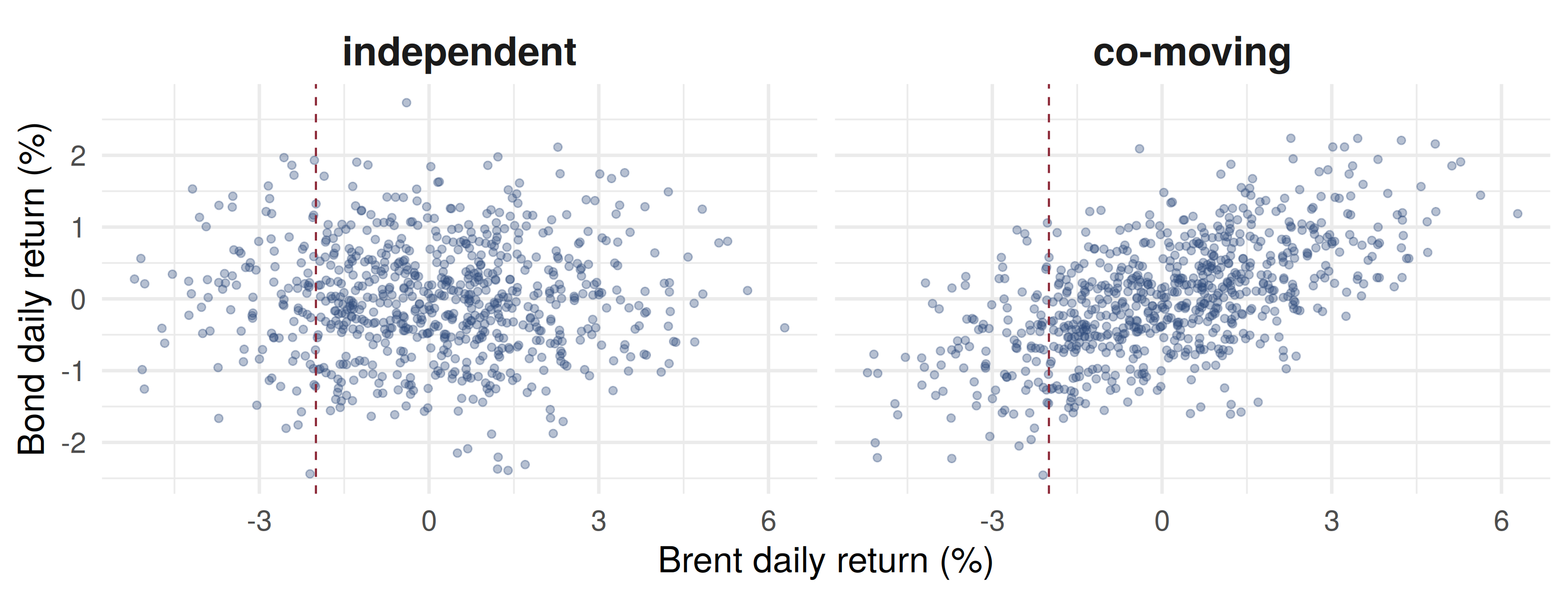
πŸ›’οΈ Co-Moving Returns

Same marginals in both panels. When Brent falls more than 2% (left of the dashes), the bond falls with probability 0.50 on the left but 0.86 on the right.

🧠 Think-Pair-Share

\(Y_1\) = tanker loadings delayed at an oil terminal today (0 or 1); \(Y_2\) = pipeline pumping-station alarms (0, 1, 2).

\(y_2 = 0\) \(y_2 = 1\) \(y_2 = 2\)
\(y_1 = 0\) 0.42 0.21 0.07
\(y_1 = 1\) 0.18 ? ?
  1. If \(Y_1\) and \(Y_2\) are independent, fill in the two missing cells.
  2. A colleague enters \(0.12\) and \(0\) instead. Independent?

βœ… Think-Pair-Share: Solution

  1. Row 0 gives \(p_1(0) = 0.70\), so \(p_1(1) = 0.30\). Independence in row 0 fixes \(p_2\): \[p_2(0) = \tfrac{0.42}{0.70} = 0.6,\quad p_2(1) = \tfrac{0.21}{0.70} = 0.3,\quad p_2(2) = 0.1\] Check \(p(1,0) = 0.3 \times 0.6 = 0.18\) βœ“. Then \(p(1,1) = 0.09\) and \(p(1,2) = 0.03\).
  1. The table still sums to 1, but \(p(1, 2) = 0\) while \(p_1(1)\,p_2(2) = 0.30 \times 0.07 = 0.021\). Dependent. A zero cell under two positive marginals always is (compare Example 5.10).

πŸ“ Quiz #1: Factorisation

\(f(y_1, y_2) = \tfrac19\, y_1^2 e^{-y_2}\) for \(0 \le y_1 \le 3\), \(y_2 > 0\), and 0 elsewhere. Are \(Y_1\), \(Y_2\) independent?

  • Yes: the support is a rectangle and \(f = g(y_1)h(y_2)\)
  • No: \(y_1\) has a finite range but \(y_2\) does not
  • Cannot say without computing both marginals
  • No: \(g(y_1) = y_1^2\) is not a density

πŸ“ Quiz #2: One Cell

In a joint table of two exporters’ monthly shipment counts, \(p(2, 0) = 0\), while \(p_1(2) = 0.2\) and \(p_2(0) = 0.4\). What follows?

  • \(Y_1\) and \(Y_2\) are dependent
  • Nothing, until the other cells are checked
  • They are independent, since \(0 \le 0.08\)
  • The table is invalid

πŸ“ Quiz #3: Using Definition 5.8

Daily losses \(Y_1\), \(Y_2\) (in million AZN) on two unrelated trading books are independent, with \(P(Y_1 \le 1) = 0.7\) and \(P(Y_2 \le 1) = 0.4\). What is \(P(Y_1 \le 1,\ Y_2 \le 1)\)?

  • \(0.28\)
  • \(0.82\)
  • \(1.10\)
  • \(0.40\)

πŸ“‹ Key Formulas

Independent if and only if
Definition 5.8 \(F(y_1, y_2) = F_1(y_1)F_2(y_2)\) for all \((y_1, y_2)\)
Theorem 5.4, discrete \(p(y_1, y_2) = p_1(y_1)p_2(y_2)\) for all pairs
Theorem 5.4, continuous \(f(y_1, y_2) = f_1(y_1)f_2(y_2)\) for all pairs
Theorem 5.5 (rectangle support) \(f(y_1, y_2) = g(y_1)h(y_2)\)
Exercise 5.43 \(f(y_1 \mid y_2) = f_1(y_1)\) whenever \(f_2(y_2) > 0\)
\(n\) variables \(F(y_1, \ldots, y_n) = F_1(y_1)\cdots F_n(y_n)\)

πŸ“‹ Summary

  • Independence means the joint distribution is the product of the marginals, everywhere

  • Tables: check every cell to prove it, find one cell to refute it; a zero cell is the quickest refutation

  • Densities: a rectangle support plus a product formula proves it (Theorem 5.5), no integration needed

  • A support that is not a rectangle proves dependence, however neatly the formula factors

  • A common factor (oil, a storm) makes variables co-move; at correlation 0.6, \(P(\text{both fall}) = 0.352\), not \(0.5 \times 0.5 = 0.25\)

πŸ“š Practice Problems

Wackerly, 7th edition

  • Exercises at the end of Β§5.4: start with 5.45, 5.48, 5.51 and 5.53, then 5.56, 5.60, 5.61, and 5.63 – 5.64

  • Return to the cash-demand example and find \(P(Y_1 < 1,\ Y_2 < 1)\) as a product of two marginal probabilities

Week 13, Problem Set 1 is open now and closes Sunday 13 December at 23:59 on WeBWorK, covering Β§5.4.

Next class (5 December): Wackerly Β§Β§5.5–5.7, expected values of functions of random variables and covariance.

πŸ™ Thank You

Dr. Samir Orujov

πŸ“§ sorujov@ada.edu.az
🏒 Building D, Room D325
πŸ•“ Office hours: Wednesday, 16:00 – 18:00

Slides and readings: sorujov.net/teaching

❓ Questions

  • Is a random variable independent of itself? When?

  • Can two variables have a triangular support and still have \(F(y_1, y_2) = F_1(y_1)F_2(y_2)\) at some points?

  • If Brent and the bond were independent, what would the right-hand scatter plot look like?