Mathematical Statistics

Chapter 5 in Review and a Comprehensive Review of Chapters 1-5

Samir Orujov, PhD

ADA University, School of Business

Information Communication Technologies Agency, Statistics Unit

2026-09-24

🎯 Learning Objectives

By the end of this lecture, you will be able to:

  • Place every tool of Chapters 1–5 on one map, and say which kind of question each one answers

  • Choose a probability model by reading what the random variable counts or measures

  • Move between joint, marginal and conditional distributions, and test independence

  • Combine Chapter 5’s covariance and linear-function results with Chapter 4’s normal model

  • Solve multi-part, exam-style problems that cross chapter boundaries

🗺️ Where We Are

Wackerly §5.12

Wednesday: the bivariate normal distribution and conditional expectations. \(E(Y_1) = E[E(Y_1 \mid Y_2)]\) (Theorem 5.14) and \(V(Y_1) = E[V(Y_1 \mid Y_2)] + V[E(Y_1 \mid Y_2)]\) (Theorem 5.15), the last new theorems of the course.

Today there is no new theory. We put the five chapters on one page, then work four exam-style problems that each cross at least two chapters.

Midterm Examination II is on 23 December: comprehensive over Chapters 1–5, with the emphasis on Chapters 4 and 5.

🧭 What Chapter 5 Was For

The book’s summary names the multinomial experiment (§5.9) as the chapter’s theme: most experiments yield several measurements \(y_1, y_2, \ldots, y_k\), observations on \(k\) random variables.

To say how likely a whole sample is, we need joint, marginal and conditional distributions.

A sample \(Y_1, \ldots, Y_n\) is usually independent with one common distribution, and independence is what lets the joint probability factor.

Wackerly’s warning: do not drown in the details. They exist to prepare inference, the subject of Math Stat II.

🗺️ The Course on One Page

Ch. The tools The question they answer
1 \(\bar{y}\), \(s^2\), \(s\); the empirical rule What does this data set look like?
2 axioms; counting; \(P(A \mid B)\); Theorems 2.5–2.9 How likely is this event?
3 \(p(y)\), \(E(Y)\), \(V(Y)\); five discrete models; \(m(t)\), \(P(t)\); Tchebysheff How is this count distributed?
4 \(F(y)\), \(f(y)\); uniform, normal, gamma, beta; \(m(t)\); Tchebysheff How is this measurement distributed?
5 joint, marginal, conditional; Cov, \(\rho\); Theorems 5.12–5.15 How do several variables behave together?

Each chapter reuses the last: Chapter 5 is Chapters 3 and 4 in two dimensions.

🔎 Which Model? Read the Variable

The variable is Model Mean
successes in \(n\) independent trials binomial \(np\)
the trial of the first (or \(r\)-th) success geometric (negative binomial) \(1/p\) (\(r/p\))
successes drawn without replacement hypergeometric \(nr/N\)
events in a fixed time or space Poisson \(\lambda\)
a time to the next (or \(\alpha\)-th) event exponential (gamma) \(\beta\) (\(\alpha\beta\))
a sum of many small effects normal \(\mu\)
a proportion on \([0, 1]\) beta \(\alpha/(\alpha + \beta)\)
counts in \(k\) categories multinomial \(np_i\)

⛓️ Chapter 5 as One Chain

Step Discrete form Result
joint \(p(y_1, y_2)\) Definition 5.1
marginal \(p_1(y_1) = \sum_{y_2} p(y_1, y_2)\) Definition 5.4
conditional \(p(y_1 \mid y_2) = p(y_1, y_2)/p_2(y_2)\) Definition 5.5
independence \(p(y_1, y_2) = p_1(y_1)p_2(y_2)\) for all pairs Theorem 5.4
covariance \(\text{Cov}(Y_1, Y_2) = E(Y_1Y_2) - \mu_1\mu_2\) Theorem 5.10
linear functions \(V(\sum a_iY_i) = \sum a_i^2V(Y_i) + 2\sum_{i<j} a_ia_j\text{Cov}(Y_i, Y_j)\) Theorem 5.12
iterated expectation \(E(Y_1) = E[E(Y_1 \mid Y_2)]\) Theorem 5.14

For continuous variables, replace each sum by an integral and \(p\) by \(f\).

📝 Problem 1: A Home-Insurance Book

An insurer in Baku holds 400 home policies. Each policy, independently, produces a claim during the year with probability 0.01. Let \(Y\) be the number of policies with a claim. A reinsurance treaty pays out if \(Y \ge 9\).

  1. Name the distribution of \(Y\), and find \(E(Y)\) and \(V(Y)\).

  2. Find \(P(Y \ge 9)\) exactly, and by the Poisson approximation.

  3. What does Tchebysheff’s theorem guarantee for \(P(|Y - 4| < 2\sigma)\)? Compare with the exact value.

Chapters 3 and 1.

✅ Problem 1: Solution

Code
n <- 400; p <- 0.01
sigma <- sqrt(n * p * (1 - p))
# |Y - 4| < 2(1.99) means 0.02 < Y < 7.98, i.e. Y = 1, ..., 7
data.frame(quantity = c("E(Y) = np", "V(Y) = npq", "P(Y >= 9), binomial",
                        "P(Y >= 9), Poisson(4)", "Tchebysheff bound, k = 2",
                        "exact P(1 <= Y <= 7)"),
           value = round(c(n * p, n * p * (1 - p), 1 - pbinom(8, n, p),
                           1 - ppois(8, 4), 1 - 1/2^2,
                           pbinom(7, n, p) - pbinom(0, n, p)), 4))
                  quantity  value
1                E(Y) = np 4.0000
2               V(Y) = npq 3.9600
3      P(Y >= 9), binomial 0.0208
4    P(Y >= 9), Poisson(4) 0.0214
5 Tchebysheff bound, k = 2 0.7500
6     exact P(1 <= Y <= 7) 0.9318
Binomial, \(\mu = 4\), \(\sigma^2 = 3.96\). The treaty is triggered with probability about 0.021; Poisson (\(\lambda = np = 4\)) misses by less than 0.001. Tchebysheff promises at least 0.75; the truth is 0.932.

📝 Problem 2: Two Loans, One Sector

A Baku bank lends to two construction firms. \(D_i = 1\) if firm \(i\) defaults within the year:

\(D_2 = 0\) \(D_2 = 1\)
\(D_1 = 0\) 0.90 0.04
\(D_1 = 1\) 0.04 0.02
  1. Find the marginal default probabilities and \(P(D_2 = 1 \mid D_1 = 1)\). Are \(D_1\) and \(D_2\) independent?

  2. Find \(\text{Cov}(D_1, D_2)\) and \(\rho\).

  3. Given that at least one firm defaults, what is the probability that firm 1 did?

✅ Problem 2: Solution

  1. \(P(D_1 = 1) = 0.04 + 0.02 = 0.06\), and likewise \(P(D_2 = 1) = 0.06\). \[P(D_2 = 1 \mid D_1 = 1) = \frac{0.02}{0.06} = 0.333 \ne 0.06,\] so they are dependent (Theorem 5.4 fails at the cell \((1, 1)\): \(0.02 \ne 0.06^2\)).

  2. \(E(D_1D_2) = P(D_1 = 1, D_2 = 1) = 0.02\), so \(\text{Cov} = 0.02 - 0.06^2 = 0.0164\), and \[\rho = \frac{0.0164}{\sqrt{0.06 \times 0.94}\sqrt{0.06 \times 0.94}} = \frac{0.0164}{0.0564} = 0.291.\]

  3. \(P(\text{at least one}) = 1 - 0.90 = 0.10\), so \(P(D_1 = 1 \mid \text{at least one}) = 0.06/0.10 = 0.6\).

💻 Problem 2, Continued: The Loss

Exposures are 80,000 and 120,000 AZN, with 45% lost on default, so \(L = 36{,}000D_1 + 54{,}000D_2\).

Code
a <- 36000; b <- 54000
v <- 0.06 * 0.94; cv <- 0.02 - 0.06^2
EL <- (a + b) * 0.06
VL <- a^2 * v + b^2 * v + 2 * a * b * cv          # Theorem 5.12
c(E_L = EL, sd_L = round(sqrt(VL)),
  sd_if_independent = round(sqrt(a^2 * v + b^2 * v)))
              E_L              sd_L sd_if_independent 
             5400             17359             15413 

The expected loss, 5,400 AZN, needs only the marginals. The spread does not: the covariance term raises the standard deviation from 15,413 to 17,359 AZN. Same-sector loans default together, and Theorem 5.12 prices that in.

📝 Problem 3: A Two-Fund Portfolio

A client puts 60% of 50,000 AZN in a bank-share fund \(A\) and 40% in an AZN bond fund \(B\). Monthly returns (%): \(\mu_A = 1.2\), \(\sigma_A = 5\); \(\mu_B = 0.8\), \(\sigma_B = 1.5\); \(\rho = -0.2\). Assume the portfolio return \(R\) is normal.

Mean (Theorem 5.12): \(E(R) = 0.6(1.2) + 0.4(0.8) = 1.04\).

Variance: \(V(R) = 0.36(25) + 0.16(2.25) + 2(0.6)(0.4)(-0.2)(5)(1.5) = 9 + 0.36 - 0.72 = 8.64\), so \(\sigma_R = 2.939\).

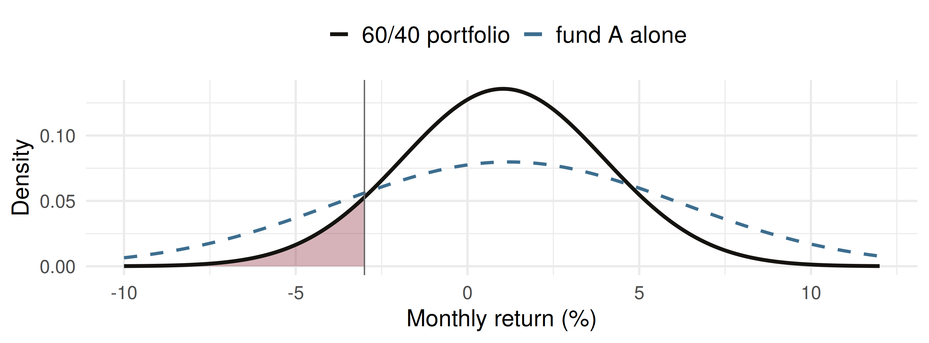
Loss of more than 3% (Chapter 4): \(P(R < -3) = P\left(Z < \frac{-3 - 1.04}{2.939}\right) = P(Z < -1.37) = 0.085\).

5% worst case: \(1.04 - 1.645(2.939) = -3.79\%\), a loss of about 1,897 AZN.

📊 Problem 3: The Picture

Shaded: \(P(R < -3) = 0.085\). Holding fund \(A\) alone, the same loss has probability \(0.200\). The negative \(\rho\) and the bond fund’s small \(\sigma\) do the work.

🧠 Think-Pair-Share: Waiting Times

A bank’s call centre has a retail line and a business line. The time to the next call is exponential, mean 4 minutes on retail (\(Y_1\)) and 6 minutes on business (\(Y_2\)), independently.

Four minutes, in pairs:

  1. Find \(P(Y_1 > 5)\). The retail line has been silent for 3 minutes: now what is the chance of 5 more?

  2. Find \(E(Y_1 + Y_2)\) and \(V(Y_1 + Y_2)\).

  3. Find \(P(Y_1 < Y_2)\), the chance that retail rings first.

✅ Think-Pair-Share: Solution

  1. \(P(Y_1 > 5) = e^{-5/4} = 0.287\), and by memorylessness \(P(Y_1 > 8 \mid Y_1 > 3) = e^{-5/4} = 0.287\) as well.

  2. Theorem 4.10 and Theorem 5.12 with \(\text{Cov} = 0\) (independence, Theorem 5.11): \[E(Y_1 + Y_2) = 4 + 6 = 10, \qquad V(Y_1 + Y_2) = 4^2 + 6^2 = 52.\]

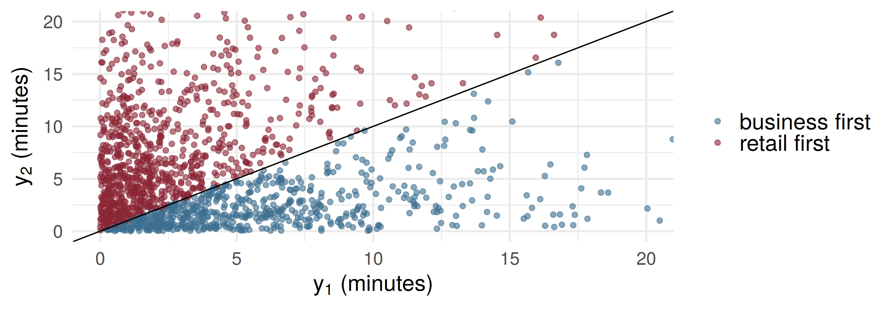
  3. Independence makes the joint density the product (Chapter 5), then integrate over \(y_1 < y_2\): \[P(Y_1 < Y_2) = \int_0^\infty \frac{1}{4}e^{-y_1/4}\int_{y_1}^\infty \frac{1}{6}e^{-y_2/6}\,dy_2\,dy_1 = \int_0^\infty \frac{1}{4}e^{-5y_1/12}\,dy_1 = \frac{1/4}{5/12} = 0.6.\]

💻 Checking Part 3 by Simulation

Code
y1 <- rexp(100000, rate = 1/4); y2 <- rexp(100000, rate = 1/6)
round(c(retail_first = mean(y1 < y2), mean_sum = mean(y1 + y2), var_sum = var(y1 + y2)), 3)
retail_first     mean_sum      var_sum 
       0.602       10.001       52.275 

100,000 simulated pairs: retail rings first about 60% of the time, as the integral said.

⚠️ Where Marks Are Lost

  • Variance of a sum without the covariance. \(V(Y_1 + Y_2) = V(Y_1) + V(Y_2)\) only when \(\text{Cov} = 0\).

  • \(\rho\) divided by variances. It is \(\text{Cov}/(\sigma_1\sigma_2)\): standard deviations.

  • Independence from one cell. One cell with \(p(y_1, y_2) = p_1(y_1)p_2(y_2)\) proves nothing; one cell without it proves dependence.

  • Zero covariance read as independence. Theorem 5.11 runs one way only.

  • Limits of integration. On a triangular support such as \(0 \le y_2 \le y_1 \le 1\), the inner limits depend on the outer variable.

  • \(\beta\) read as a rate. In Wackerly, the exponential with parameter \(\beta\) has mean \(\beta\).

📝 Quiz #1: Default Across the Cycle

A borrower’s default probability is 0.02 in an expansion and 0.08 in a recession. The economy is in expansion with probability 0.7. What is the unconditional default probability?

  • \(0.038\)
  • \(0.050\)
  • \(0.080\)
  • \(0.0016\)

📝 Quiz #2: A Hedged Position

A trader is long \(Y_1\) and short \(Y_2\), with \(V(Y_1) = 4\), \(V(Y_2) = 9\) and \(\text{Cov}(Y_1, Y_2) = 3\). What is \(V(Y_1 - Y_2)\)?

  • \(7\)
  • \(13\)
  • \(19\)
  • \(-5\)

📝 Quiz #3: Which Model?

On the retail line above (exponential, mean 4 minutes), what is the distribution of the time until the third call?

  • Gamma with \(\alpha = 3\), \(\beta = 4\): mean 12 minutes
  • Exponential with mean 12 minutes
  • Poisson with \(\lambda = 3\)
  • Geometric with \(p = 1/4\)

📋 Key Formulas

Statement
Theorem 2.9 (Bayes) \(P(B_j \mid A) = P(A \mid B_j)P(B_j) / \sum_i P(A \mid B_i)P(B_i)\)
Tchebysheff \(P(\lvert Y - \mu \rvert < k\sigma) \ge 1 - 1/k^2\)
Theorem 5.4 independent iff \(p(y_1, y_2) = p_1(y_1)p_2(y_2)\) for all pairs
Theorem 5.10 \(\text{Cov}(Y_1, Y_2) = E(Y_1Y_2) - \mu_1\mu_2\), \(\quad \rho = \text{Cov}/(\sigma_1\sigma_2)\)
Theorem 5.12 \(V(\sum a_iY_i) = \sum a_i^2V(Y_i) + 2\sum_{i<j}a_ia_j\text{Cov}(Y_i, Y_j)\)
Theorem 5.14 \(E(Y_1) = E[E(Y_1 \mid Y_2)]\)
Theorem 5.15 \(V(Y_1) = E[V(Y_1 \mid Y_2)] + V[E(Y_1 \mid Y_2)]\)

📋 Summary

  • Chapters 1–5 are one argument: events, then counts, then measurements, then several variables at once

  • Choose the model by reading what the variable counts or measures, before any formula

  • Chapter 5’s chain: joint, marginal, conditional, independence, covariance, linear functions, iterated expectation

  • Means of sums need only marginals; variances of sums need covariances

  • Most exam problems join two chapters: a Chapter 5 result feeding a Chapter 3 or 4 model

  • Wackerly’s advice for the midterm: master the ideas, and let the details serve them

📚 Practice Problems

Wackerly, 7th edition

  • Chapter 5 Supplementary Exercises 5.144 – 5.167; start with 5.145, 5.147, 5.148, 5.150, 5.153, 5.158 and 5.161

  • The Supplementary Exercises of Chapters 3 and 4, for the models in the map

  • Redo Problem 3 with \(\rho = +0.2\): how much does \(\sigma_R\) rise?

Week 15, Problem Set 2 is open now and closes Sunday 27 December at 23:59 on WeBWorK, covering Chapters 1–5 in review (§5.12).

Next class: Midterm Examination II, 23 December, comprehensive over Chapters 1–5.

🙏 Thank You

Dr. Samir Orujov

📧 sorujov@ada.edu.az
🏢 Building D, Room D325
🕓 Office hours: Wednesday, 16:00 – 18:00

Slides and readings: sorujov.net/teaching

❓ Questions

  • In Problem 2, what would the four cells have to be for \(D_1\) and \(D_2\) to be independent, with both marginals still 0.06?

  • In Problem 1, why is Tchebysheff’s bound so far below the exact 0.932, and when would you still prefer it?

  • In Problem 3, normality of \(R\) was assumed. What would you assume about the pair of fund returns to justify it?