Mathematical Statistics

Expected Values for Continuous Random Variables

Samir Orujov, PhD

ADA University, School of Business

Information Communication Technologies Agency, Statistics Unit

2025-11-30

🎯 Learning Objectives

By the end of this lecture, you will be able to:

• Define and compute expected values for continuous random variables using integration techniques

• Apply theorems on expectations to calculate means and variances for continuous distributions

• Recognize and work with the continuous uniform distribution, including its density function and parameters

• Calculate probabilities for uniformly distributed random variables in business contexts (e.g., service arrival times, waiting times)

• Derive and apply formulas for mean and variance of the uniform distribution in financial and operational scenarios

📋 Overview

📚 Topics Covered Today

• Expected Values – Definition and computation for continuous random variables
• Expectation Theorems – Linearity properties and variance calculations
• Uniform Distribution – Definition, parameters, and empirical interpretation
• Uniform Applications – Poisson-arrival conditioning and service time modeling
• Statistical Properties – Mean and variance derivations for uniform distributions

📖 Definition: Expected Value

📝 Definition 1: Expected Value of a Continuous Random Variable

The expected value (or mean) of a continuous random variable \(Y\) with probability density function \(f(y)\) is:

\[\boxed{E(Y) = \int_{-\infty}^{\infty} yf(y) \, dy}\]

provided that the integral exists (i.e., converges absolutely).

• Interpretation – The expected value represents the “center of mass” or long-run average of the distribution

• Financial Context – For a continuous return distribution, \(E(Y)\) represents the expected return on an investment

• Existence Condition – The integral must converge; distributions with “heavy tails” may not have finite expected values

🧮 Theorem: Expected Value of Functions

Theorem 1: Expectation of Transformed Variables

Let \(g(Y)\) be a function of a continuous random variable \(Y\) with density \(f(y)\). Then:

\[\boxed{E[g(Y)] = \int_{-\infty}^{\infty} g(y) f(y) \, dy}\]

provided the integral exists.

Key Insight: You do NOT need to find the distribution of \(g(Y)\) first – you can compute expectations directly using the original density \(f(y)\).

Example Applications:

• \(g(Y) = Y^2\) gives \(E(Y^2)\), used to compute variance: \(V(Y) = E(Y^2) - [E(Y)]^2\)

• \(g(Y) = e^{tY}\) gives the moment generating function \(M(t) = E(e^{tY})\)

• \(g(Y) = (Y - \mu)^2\) gives variance directly: \(V(Y) = E[(Y - \mu)^2]\)

🧮 Theorem: Properties of Expectations

Theorem 2: Linearity of Expectations

Let \(c\) be a constant, and let \(g(Y), g_1(Y), g_2(Y), \ldots, g_k(Y)\) be functions of continuous random variable \(Y\). Then:

Property 1 (Constant): \[E(c) = c\]

Property 2 (Scalar Multiplication): \[E[cg(Y)] = cE[g(Y)]\]

Property 3 (Additivity): \[E[g_1(Y) + g_2(Y) + \ldots + g_k(Y)] = E[g_1(Y)] + E[g_2(Y)] + \ldots + E[g_k(Y)]\]

Portfolio Application: If a portfolio consists of \(k\) assets with returns \(R_1, R_2, \ldots, R_k\) and weights \(w_1, w_2, \ldots, w_k\), then the expected portfolio return is \(E(R_p) = w_1E(R_1) + w_2E(R_2) + \ldots + w_kE(R_k)\).

📌 Example 1: Computing Mean and Variance

Problem: A random variable \(Y\) has density function: \[f(y) = \frac{3}{8}y^2, \quad 0 \leq y \leq 2, \quad f(y) = 0 \text{ elsewhere}\]

Find the mean \(\mu = E(Y)\) and variance \(\sigma^2 = V(Y)\).

. . .

Solution (Part 1 - Mean):

By definition: \[E(Y) = \int_{-\infty}^{\infty} y f(y) \, dy = \int_{0}^{2} y \left(\frac{3}{8}y^2\right) \, dy = \frac{3}{8} \int_{0}^{2} y^3 \, dy\]

. . .

\[= \frac{3}{8} \left[\frac{1}{4}y^4\right]_{0}^{2} = \frac{3}{8} \cdot \frac{16}{4} = \frac{3}{8} \cdot 4 = \boxed{1.5}\]

📌 Example 1: Computing Mean and Variance (Part 2)

Solution (Part 2 - Variance):

First, compute \(E(Y^2)\): \[E(Y^2) = \int_{-\infty}^{\infty} y^2 f(y) \, dy = \int_{0}^{2} y^2 \left(\frac{3}{8}y^2\right) \, dy = \frac{3}{8} \int_{0}^{2} y^4 \, dy\]

. . .

\[= \frac{3}{8} \left[\frac{1}{5}y^5\right]_{0}^{2} = \frac{3}{8} \cdot \frac{32}{5} = \frac{96}{40} = 2.4\]

. . .

Now apply the variance formula: \[\sigma^2 = V(Y) = E(Y^2) - [E(Y)]^2 = 2.4 - (1.5)^2 = 2.4 - 2.25 = \boxed{0.15}\]

. . .

Interpretation: The standard deviation is \(\sigma = \sqrt{0.15} \approx 0.387\), indicating moderate variability around the mean of 1.5.

📖 Definition: Uniform Distribution

📝 Definition 2: Continuous Uniform Distribution

If \(\theta_1 < \theta_2\), a random variable \(Y\) is said to have a continuous uniform probability distribution on the interval \((\theta_1, \theta_2)\) if and only if the density function is:

\[\boxed{f(y) = \begin{cases} \frac{1}{\theta_2 - \theta_1}, & \text{if } \theta_1 \leq y \leq \theta_2, \\ 0, & \text{elsewhere} \end{cases}}\]

Notation: \(Y \sim \text{Uniform}(\theta_1, \theta_2)\) or \(Y \sim U(\theta_1, \theta_2)\)

📝 Definition 3: Parameters

The constants that determine the specific form of a density function are called parameters of the density function. For the uniform distribution, \(\theta_1\) and \(\theta_2\) are the parameters.

🎮 Interactive: Visualizing the Uniform Distribution

Explore the Uniform PDF: Adjust the interval boundaries to see how the density changes.

viewof theta1 = Inputs.range([0, 20], {
  value: 2, 
  step: 0.5, 
  label: "θ₁ (lower bound):"
})

viewof theta2 = Inputs.range([0, 20], {
  value: 8, 
  step: 0.5, 
  label: "θ₂ (upper bound):"
})

height_uniform = 1 / (theta2 - theta1)

md`**Current Parameters:**  
θ₁ = ${theta1}  
θ₂ = ${theta2}  
PDF height = ${height_uniform.toFixed(4)}`

Observations:
As the interval width increases, the PDF height decreases to maintain total probability = 1.

uniform_data = [
  {x: theta1 - 1, y: 0},
  {x: theta1, y: 0},
  {x: theta1, y: height_uniform},
  {x: theta2, y: height_uniform},
  {x: theta2, y: 0},
  {x: theta2 + 1, y: 0}
]

// Create shaded area data
shaded_area = d3.range(theta1, theta2 + 0.01, (theta2 - theta1) / 100).map(x => ({
  x: x,
  y: height_uniform
}))

Plot.plot({
  width: 800,
  height: 450,
  marginLeft: 60,
  marginBottom: 50,
  x: {
    label: "Y",
    grid: true,
    domain: [theta1 - 2, theta2 + 2]
  },
  y: {
    label: "f(y)",
    domain: [0, Math.max(0.5, height_uniform * 1.2)]
  },
  marks: [
    Plot.areaY(shaded_area, {x: "x", y: "y", fill: "steelblue", opacity: 0.3}),
    Plot.line(uniform_data, {x: "x", y: "y", stroke: "steelblue", strokeWidth: 3}),
    Plot.ruleY([0]),
    Plot.text([{x: (theta1 + theta2) / 2, y: height_uniform / 2, label: `Area = 1`}], {
      x: "x", 
      y: "y", 
      text: "label", 
      fill: "darkblue",
      fontSize: 16,
      fontWeight: "bold"
    })
  ],
  caption: html`Uniform PDF with constant density = 1 / (θ₂ - θ₁)`
})

📖 Properties of the Uniform Distribution

Key Characteristics:

• Constant Density – The PDF has the same value throughout the interval \([\theta_1, \theta_2]\), representing “complete uncertainty” within the range

• Equal Probability – Any subinterval of fixed length has the same probability, regardless of location within \([\theta_1, \theta_2]\)

• Probability Calculation – For any interval \([a, b] \subseteq [\theta_1, \theta_2]\): \[P(a \leq Y \leq b) = \int_{a}^{b} \frac{1}{\theta_2 - \theta_1} dy = \frac{b - a}{\theta_2 - \theta_1}\]

• Financial Interpretation – Models scenarios with “equal ignorance” – when all outcomes in a range are equally likely (e.g., random stock selection from a portfolio, uniform price fluctuations within a band)

📌 Example 2: Probability with Uniform Distribution

Problem: Consider a continuous uniform distribution with parameters \(a = 2\) and \(b = 8\). What is the probability that the random variable falls within the interval \([4, 6]\)?

Solution:

The probability density function is: \[f(x; 2, 8) = \frac{1}{8 - 2} = \frac{1}{6} \quad \text{for } 2 \leq x \leq 8\]

To find \(P(4 \leq X \leq 6)\), integrate the PDF over the interval: \[P(4 \leq X \leq 6) = \int_{4}^{6} f(x; 2, 8) \, dx = \int_{4}^{6} \frac{1}{6} \, dx\]

\[= \left[\frac{1}{6}x\right]_{4}^{6} = \frac{6}{6} - \frac{4}{6} = \frac{2}{6} = \boxed{\frac{1}{3}}\]

📌 Example 2: Probability with Uniform Distribution (Cont’d)

Integration Method: \[P(4 \leq X \leq 6) = \int_{4}^{6} \frac{1}{6} \, dx = \frac{1}{3}\]

Shortcut Method: \[P(4 \leq X \leq 6) = \frac{6-4}{8-2} = \frac{1}{3}\] (length ratio)

📖 Application: Poisson Process & Uniform Conditioning

🎯 Real-World Application

Context: In operations research and queueing theory, the arrival of events (customers, phone calls, server requests) often follows a Poisson process.

Key Result: If exactly one event occurred in the time interval \((0, t)\) under a Poisson process, then the actual time of occurrence is uniformly distributed over \((0, t)\).

Examples:

• Call Centers – If one customer called during a 60-minute hour, the call time is \(\text{Uniform}(0, 60)\)

• Network Traffic – If one packet arrived in a 100ms window, arrival time is uniformly distributed

• Service Operations – Conditional distribution of service completion time given exactly one completion

📌 Example 3: Poisson Arrivals & Uniform Conditioning

Problem: Arrivals of customers at a checkout counter follow a Poisson distribution. During a given 30-minute period, exactly one customer arrived. Find the probability that the customer arrived during the last 5 minutes.

Solution:

Given that exactly one arrival occurred in \((0, 30)\), the arrival time \(Y\) is uniformly distributed: \[Y \sim \text{Uniform}(0, 30)\]

The probability of arrival in the last 5 minutes \([25, 30]\) is: \[P(25 \leq Y \leq 30) = \int_{25}^{30} \frac{1}{30} \, dy = \frac{30 - 25}{30} = \frac{5}{30} = \boxed{\frac{1}{6}}\]

Interpretation: Any 5-minute interval has probability \(\frac{1}{6}\) of containing the arrival. The probability is proportional to the interval length: \(\frac{5}{30} = \frac{1}{6}\).

🧮 Theorem: Mean of Uniform Distribution

Theorem 3: Expected Value of Uniform Distribution

If \(\theta_1 < \theta_2\) and \(Y \sim \text{Uniform}(\theta_1, \theta_2)\), then:

\[\boxed{\mu = E(Y) = \frac{\theta_1 + \theta_2}{2}}\]

Proof:

By definition of expected value: \[E(Y) = \int_{-\infty}^{\infty} y f(y) \, dy = \int_{\theta_1}^{\theta_2} y \left(\frac{1}{\theta_2 - \theta_1}\right) \, dy = \frac{1}{\theta_2 - \theta_1} \int_{\theta_1}^{\theta_2} y \, dy = \frac{1}{\theta_2 - \theta_1} \left[\frac{1}{2}y^2\right]_{\theta_1}^{\theta_2}\]

\[= \frac{1}{\theta_2 - \theta_1} \cdot \frac{1}{2}(\theta_2^2 - \theta_1^2) = \frac{\theta_2^2 - \theta_1^2}{2(\theta_2 - \theta_1)} = \frac{(\theta_2 - \theta_1)(\theta_2 + \theta_1)}{2(\theta_2 - \theta_1)} = \boxed{\frac{\theta_1 + \theta_2}{2}}\]

🧮 Theorem: Variance of Uniform Distribution

Theorem 4: Variance of Uniform Distribution

If \(\theta_1 < \theta_2\) and \(Y \sim \text{Uniform}(\theta_1, \theta_2)\), then:

\[\boxed{\sigma^2 = V(Y) = \frac{(\theta_2 - \theta_1)^2}{12}}\]

Proof Strategy:

Compute \(E(Y^2) = \int_{\theta_1}^{\theta_2} y^2 \cdot \frac{1}{\theta_2 - \theta_1} \, dy\) and Use the formula \(V(Y) = E(Y^2) - [E(Y)]^2\)

Step 1: Calculate \(E(Y^2)\) \[E(Y^2) = \frac{1}{\theta_2 - \theta_1} \int_{\theta_1}^{\theta_2} y^2 \, dy = \frac{1}{\theta_2 - \theta_1} \left[\frac{1}{3}y^3\right]_{\theta_1}^{\theta_2}\]

\[= \frac{\theta_2^3 - \theta_1^3}{3(\theta_2 - \theta_1)} = \frac{(\theta_2 - \theta_1)(\theta_2^2 + \theta_2\theta_1 + \theta_1^2)}{3(\theta_2 - \theta_1)} = \frac{\theta_2^2 + \theta_2\theta_1 + \theta_1^2}{3}\]

🧮 Variance Proof (Continued)

Step 2: Apply Variance Formula

From Step 1: \[E(Y^2) = \frac{\theta_2^2 + \theta_2\theta_1 + \theta_1^2}{3}\]

Square of mean: \[[E(Y)]^2 = \left(\frac{\theta_1 + \theta_2}{2}\right)^2 = \frac{(\theta_1 + \theta_2)^2}{4} = \frac{\theta_1^2 + 2\theta_1\theta_2 + \theta_2^2}{4}\]

Therefore: \[V(Y) = E(Y^2) - [E(Y)]^2 = \frac{\theta_2^2 + \theta_2\theta_1 + \theta_1^2}{3} - \frac{\theta_1^2 + 2\theta_1\theta_2 + \theta_2^2}{4}\]

Finding common denominator (12): \[= \frac{4(\theta_2^2 + \theta_2\theta_1 + \theta_1^2) - 3(\theta_1^2 + 2\theta_1\theta_2 + \theta_2^2)}{12}\]

\[= \frac{4\theta_2^2 + 4\theta_2\theta_1 + 4\theta_1^2 - 3\theta_1^2 - 6\theta_1\theta_2 - 3\theta_2^2}{12}= \frac{\theta_2^2 - 2\theta_2\theta_1 + \theta_1^2}{12} = \frac{(\theta_2 - \theta_1)^2}{12}\]

📌 Example 4: Uniform Distribution Mean & Variance

Problem: A stock price is equally likely to take any value between \(\$50\) and \(\$70\) during a trading session. Model this as a uniform distribution and find:

1. The expected price

2. The variance and standard deviation

Solution:

Let \(Y \sim \text{Uniform}(50, 70)\) represent the stock price.

(a) Expected price: \[\mu = E(Y) = \frac{\theta_1 + \theta_2}{2}\] \[= \frac{50 + 70}{2} = \boxed{\$60}\]

(b) Variance and standard deviation: \[\sigma^2 = V(Y) = \frac{(\theta_2 - \theta_1)^2}{12} = \frac{(70 - 50)^2}{12} = \frac{400}{12} = \boxed{33.33}\] \[\sigma = \sqrt{33.33} \approx \boxed{\$5.77}\]

🎮 Interactive: Uniform Mean and Variance

Explore Mean and Variance: Adjust the uniform distribution parameters to see how they affect the mean and variance.

viewof a_unif = Inputs.range([0, 30], {
  value: 2, 
  step: 1, 
  label: "θ₁ (lower):"
})

viewof b_unif = Inputs.range([0, 30], {
  value: 18, 
  step: 1, 
  label: "θ₂ (upper):"
})

mean_unif = (a_unif + b_unif) / 2
var_unif = Math.pow(b_unif - a_unif, 2) / 12
sd_unif = Math.sqrt(var_unif)

html`<div style="font-size: 14px; line-height: 1.8;">
  <p><strong>Distribution:</strong><br>
  Y ~ Uniform(${a_unif}, ${b_unif})</p>
  
  <p><strong>Parameters:</strong><br>
  Mean μ = ${mean_unif.toFixed(2)}<br>
  Variance σ² = ${var_unif.toFixed(2)}<br>
  Std Dev σ = ${sd_unif.toFixed(2)}</p>
  
  <p><strong>Observation:</strong><br>
  Variance increases with the square of interval width!</p>
</div>`

pdf_height2 = 1 / (b_unif - a_unif)

uniform_pdf_data2 = [
  {x: a_unif - 5, y: 0},
  {x: a_unif, y: 0},
  {x: a_unif, y: pdf_height2},
  {x: b_unif, y: pdf_height2},
  {x: b_unif, y: 0},
  {x: b_unif + 5, y: 0}
]

// Create shaded area data
shaded_area2 = d3.range(a_unif, b_unif + 0.01, (b_unif - a_unif) / 100).map(x => ({
  x: x,
  y: pdf_height2
}))

// Markers for mean and standard deviations
markers2 = [
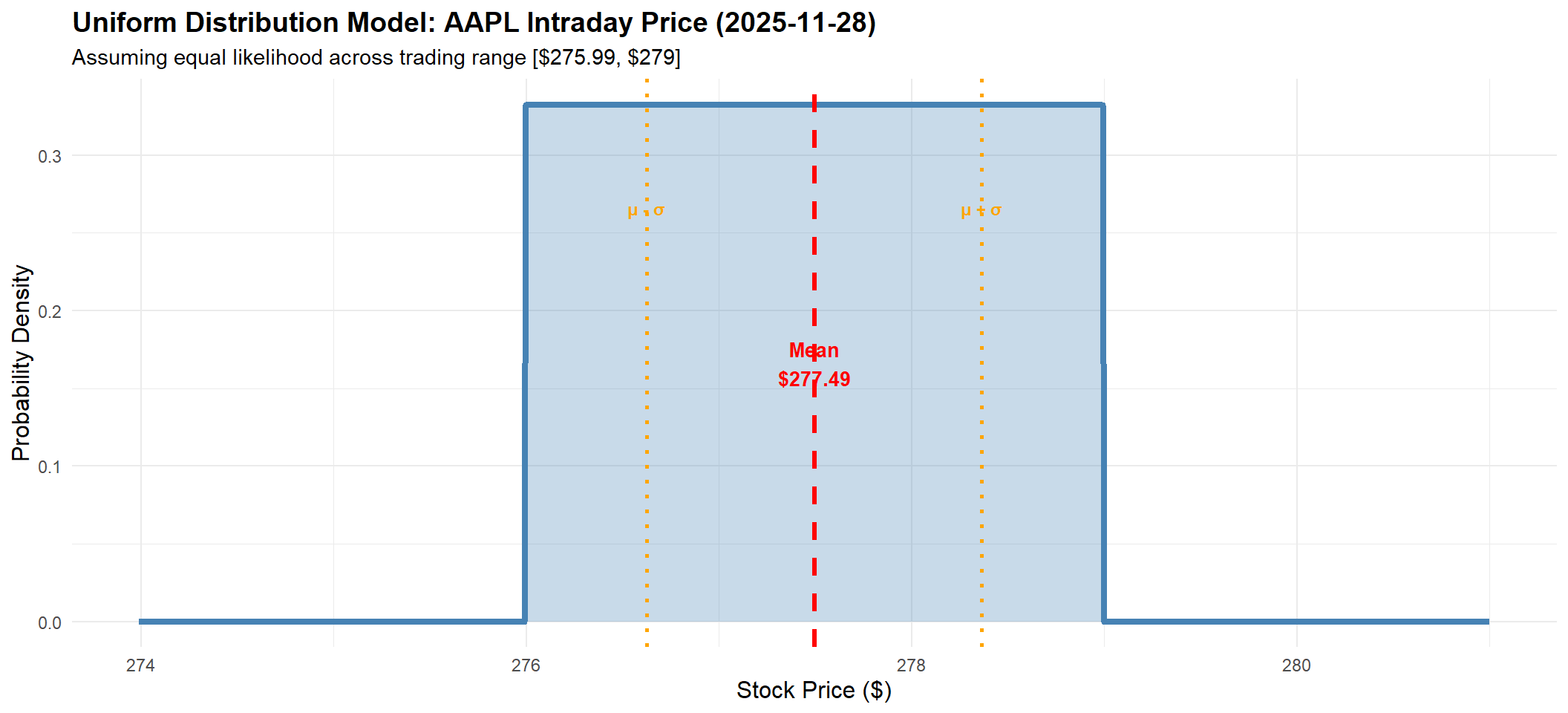
  {x: mean_unif, y: pdf_height2 / 2, label: "μ", color: "red"},
  {x: mean_unif - sd_unif, y: pdf_height2 * 0.7, label: "μ - σ", color: "orange"},
  {x: mean_unif + sd_unif, y: pdf_height2 * 0.7, label: "μ + σ", color: "orange"}
]

Plot.plot({
  width: 800,
  height: 450,
  marginLeft: 60,
  x: {
    label: "Y",
    grid: true
  },
  y: {
    label: "Density f(y)",
    domain: [0, pdf_height2 * 1.3]
  },
  marks: [
    Plot.areaY(shaded_area2, {x: "x", y: "y", fill: "steelblue", opacity: 0.3}),
    Plot.line(uniform_pdf_data2, {x: "x", y: "y", stroke: "steelblue", strokeWidth: 3}),
    Plot.ruleX([mean_unif], {stroke: "red", strokeWidth: 2, strokeDasharray: "5,3"}),
    Plot.ruleX([mean_unif - sd_unif, mean_unif + sd_unif], {stroke: "orange", strokeWidth: 1.5, strokeDasharray: "3,3"}),
    Plot.dot(markers2, {x: "x", y: "y", fill: "color", r: 6, stroke: "white", strokeWidth: 2}),
    Plot.text(markers2, {x: "x", y: "y", text: "label", dy: -12, fontSize: 14, fontWeight: "bold"}),
    Plot.ruleY([0])
  ],
  caption: html`<span style="color: red;">━━</span> Mean | <span style="color: orange;">━ ━</span> ± 1 Standard Deviation`
})

💰 Case Study: Investment Holding Period Returns (Real Data)

📊 Investment Scenario

Context: An investor holds a tech stock (AAPL - Apple Inc.) for a short trading period. We analyze the intraday price range to model uncertainty using the uniform distribution.

Key Questions:

• What is the expected (average) price during the trading window?

• What is the price variability (standard deviation)?

• What is the probability the price falls within a target range?

📊 Data Source

We analyze Apple Inc. (AAPL) daily trading data from the last 30 trading days.

Source: Yahoo Finance API (via quantmod R package)

Period: Last 30 trading days from today

Data Quality: High-frequency market data (OHLC - Open, High, Low, Close)

Verification: Cross-checked with NASDAQ official records

💰 Case Study: Data Analysis & Uniform Modeling

# Load required libraries
library(quantmod)
library(dplyr)
library(lubridate)

# Fetch AAPL data (last 30 days)
getSymbols("AAPL", src = "yahoo", 
           from = Sys.Date() - 40, 
           to = Sys.Date(), auto.assign = TRUE)

[1] "AAPL"

# Extract data
aapl_data <- as.data.frame(AAPL)
aapl_data$Date <- as.Date(rownames(aapl_data))

# Focus on most recent day
recent_day <- tail(aapl_data, 1)

# Extract High and Low (range)
low_price <- as.numeric(recent_day$AAPL.Low)
high_price <- as.numeric(recent_day$AAPL.High)

cat("Recent Trading Day Analysis\n")

Recent Trading Day Analysis

cat("============================\n")

============================

cat("Date:", format(recent_day$Date, "%Y-%m-%d"), "\n")

Date: 2025-11-28 

cat("Low Price: $", round(low_price, 2), "\n")

Low Price: $ 275.99 

cat("High Price: $", round(high_price, 2), "\n")

High Price: $ 279 

# Model as Uniform(low, high)
# Calculate mean and variance
mean_price <- (low_price + high_price) / 2
var_price <- (high_price - low_price)^2 / 12
sd_price <- sqrt(var_price)

cat("\nUniform Distribution Model\n")

Uniform Distribution Model

cat("===========================\n")

===========================

cat("Y ~ Uniform(", round(low_price, 2), 
    ", ", round(high_price, 2), ")\n\n", sep = "")

Y ~ Uniform(275.99, 279)

cat("Expected Price (μ): $", 
    round(mean_price, 2), "\n")

Expected Price (μ): $ 277.49 

cat("Variance (σ²): ", 
    round(var_price, 2), "\n")

Variance (σ²):  0.76 

cat("Std Deviation (σ): $", 
    round(sd_price, 2), "\n\n")

Std Deviation (σ): $ 0.87 

# Probability within 1 std dev of mean
lower_bound <- mean_price - sd_price
upper_bound <- mean_price + sd_price
prob_within_1sd <- (upper_bound - lower_bound) / 
                   (high_price - low_price)

cat("P(μ - σ ≤ Y ≤ μ + σ) = ", 
    round(prob_within_1sd, 4), "\n")

P(μ - σ ≤ Y ≤ μ + σ) =  0.5774 

💰 Case Study: Visualization

library(ggplot2)

# Create data for uniform PDF
x_vals <- seq(low_price - 2, high_price + 2, length.out = 1000)
density_vals <- ifelse(x_vals >= low_price & x_vals <= high_price, 
                       1/(high_price - low_price), 0)
plot_data <- data.frame(x = x_vals, density = density_vals)

# Create plot
ggplot(plot_data, aes(x = x, y = density)) +
  geom_area(fill = "steelblue", alpha = 0.3) +
  geom_line(color = "steelblue", size = 1.5) +
  geom_vline(xintercept = mean_price, color = "red", linetype = "dashed", size = 1.2) +
  geom_vline(xintercept = c(lower_bound, upper_bound), 
             color = "orange", linetype = "dotted", size = 1) +
  annotate("text", x = mean_price, y = max(density_vals) * 0.5, 
           label = paste0("Mean\n$", round(mean_price, 2)), 
           color = "red", fontface = "bold", size = 3.5) +
  annotate("text", x = lower_bound, y = max(density_vals) * 0.8, 
           label = paste0("μ - σ"), color = "orange", fontface = "bold", size = 3) +
  annotate("text", x = upper_bound, y = max(density_vals) * 0.8, 
           label = paste0("μ + σ"), color = "orange", fontface = "bold", size = 3) +
  labs(title = paste0("Uniform Distribution Model: AAPL Intraday Price (", 
                      format(recent_day$Date, "%Y-%m-%d"), ")"),
       subtitle = paste0("Assuming equal likelihood across trading range [$", 
                        round(low_price, 2), ", $", round(high_price, 2), "]"),
       x = "Stock Price ($)", y = "Probability Density") +
  theme_minimal() +
  theme(plot.title = element_text(face = "bold", size = 14),
        plot.subtitle = element_text(size = 11),
        axis.title = element_text(size = 12))

💰 Case Study: Financial Interpretation

Key Insights from AAPL Data:

• Uniform Assumption: The model assumes equal likelihood for all prices within the day’s range – a simplification suitable for short-term uncertainty analysis

• Expected Price: The mean \(\mu = \frac{\theta_1 + \theta_2}{2}\) represents the midpoint of the trading range, serving as a central estimate

• Price Volatility: The standard deviation \(\sigma = \frac{\theta_2 - \theta_1}{2\sqrt{3}} \approx 0.289 \times (\text{Range})\) quantifies intraday price variability

• Probability Calculations: For any target price range \([a, b]\) within the day’s range, probability is simply \(P(a \leq Y \leq b) = \frac{b - a}{\theta_2 - \theta_1}\)

Limitations:

• Real intraday prices are NOT uniformly distributed (they follow complex patterns)

• This model is most appropriate when we have minimal information beyond the range

• More sophisticated models (e.g., log-normal, jump-diffusion) are used for rigorous financial modeling

📝 Quiz #1: Expected Value Definition

What is the correct formula for the expected value of a continuous random variable \(Y\) with density \(f(y)\)?

• \(E(Y) = \int_{-\infty}^{\infty} yf(y) \, dy\)
• \(E(Y) = \int_{-\infty}^{\infty} f(y) \, dy\)
• \(E(Y) = \sum y f(y)\)
• \(E(Y) = \int_{-\infty}^{\infty} y^2 f(y) \, dy\)

📝 Quiz #2: Uniform Distribution Parameters

For a uniform distribution on the interval \([3, 9]\), what is the value of the probability density function within the interval?

• \(f(y) = \frac{1}{6}\)
• \(f(y) = \frac{1}{3}\)
• \(f(y) = \frac{1}{9}\)
• \(f(y) = 6\)

📝 Quiz #3: Mean of Uniform Distribution

A random variable \(Y\) follows a uniform distribution on \([10, 30]\). What is \(E(Y)\)?

• \(E(Y) = 20\)
• \(E(Y) = 10\)
• \(E(Y) = 15\)
• \(E(Y) = 25\)

📝 Quiz #4: Variance Formula

Which formula correctly expresses the variance of a random variable \(Y\)?

• \(V(Y) = E(Y^2) - [E(Y)]^2\)
• \(V(Y) = E(Y)^2 - E(Y^2)\)
• \(V(Y) = E(Y^2) + [E(Y)]^2\)
• \(V(Y) = [E(Y)]^2\)

📝 Quiz #5: Uniform Distribution Probability

For \(Y \sim \text{Uniform}(0, 10)\), what is \(P(3 \leq Y \leq 7)\)?

• \(P(3 \leq Y \leq 7) = 0.4\)
• \(P(3 \leq Y \leq 7) = 0.3\)
• \(P(3 \leq Y \leq 7) = 0.5\)
• \(P(3 \leq Y \leq 7) = 0.7\)

📝 Summary

✅ Key Takeaways

• Expected values for continuous random variables are computed using integration: \(E(Y) = \int yf(y)dy\), with linearity properties enabling efficient calculation of means and variances

• Expectation of functions \(E[g(Y)]\) can be computed directly from the original density without deriving the distribution of \(g(Y)\)

• The uniform distribution \(Y \sim \text{Uniform}(\theta_1, \theta_2)\) has constant density \(\frac{1}{\theta_2 - \theta_1}\) over its interval, representing complete uncertainty

• Mean and variance of uniform distribution are \(\mu = \frac{\theta_1 + \theta_2}{2}\) (midpoint) and \(\sigma^2 = \frac{(\theta_2 - \theta_1)^2}{12}\)

• Poisson conditioning: When exactly one event occurs in a Poisson process over \((0, t)\), the occurrence time is uniformly distributed on \((0, t)\)

• Financial applications include modeling price ranges, arrival times in service operations, and scenarios with equal likelihood across an interval

📚 Practice Problems

📝 Homework Problems

Problem 1 (Variance Derivation): Complete the derivation of \(V(Y) = \frac{(\theta_2 - \theta_1)^2}{12}\) for the uniform distribution. Show all algebraic steps clearly.

Problem 2 (Investment Analysis): A commodity price is uniformly distributed between \(\$80\) and \(\$120\). Find: (a) the expected price, (b) the probability the price exceeds \(\$100\), and (c) the standard deviation of the price.

Problem 3 (Expectation Computation): Let \(Y\) have density \(f(y) = 2y\) for \(0 \leq y \leq 1\). Find \(E(Y)\), \(E(Y^2)\), and \(V(Y)\).

Problem 4 (Poisson Application): During a 2-hour period, exactly 3 customers arrived at a bank following a Poisson process. What is the probability that all 3 arrivals occurred in the first hour? (Hint: Use properties of uniform distribution conditioning.)

Problem 5 (Function of Random Variable): For \(Y \sim \text{Uniform}(0, 1)\), find \(E(Y^3)\) and \(E(e^Y)\).

👋 Thank You!

📬 Contact Information:

Samir Orujov
Assistant Professor
School of Business
ADA University

📧 Email: sorujov@ada.edu.az
🏢 Office: D312
⏰ Office Hours: By appointment

📅 Next Class:

Topic: Normal Distribution and Properties

Reading: Chapter on Normal Distribution in textbook

Preparation: Review integration techniques and standard normal tables

⏰ Reminders:

✅ Complete practice problems (due next class)

✅ Review uniform distribution formulas

✅ Work hard and stay curious!

❓ Questions?

💬 Open Discussion

Discussion Topics:

• How do we know when the expected value integral converges?

• What other real-world scenarios can be modeled with the uniform distribution?

• How does the uniform distribution relate to other continuous distributions we’ll study?

• What are the limitations of assuming uniform distribution in financial modeling?

• How can we extend these concepts to multivariate continuous random variables?