Mathematical Statistics

The Gamma Probability Distribution

Samir Orujov, PhD

ADA University, School of Business

Information Communication Technologies Agency, Statistics Unit

2025-12-06

🎯 Learning Objectives

By the end of this lecture, you will be able to:

Define the gamma distribution and identify its shape parameter ($\alpha$) and scale parameter ($\beta$), and understand how they affect distribution characteristics
Compute probabilities, expected values, and variances for gamma-distributed random variables, including exponential and chi-square special cases
Apply the exponential distribution to model waiting times and understand the memoryless property in reliability and financial risk contexts
Use the chi-square distribution ($\chi^2$) for statistical inference, hypothesis testing, and volatility modeling in finance
Solve real-world problems involving skewed distributions in insurance claims, component lifetimes, income distributions, and water demand forecasting

📋 Overview

📚 Topics Covered Today

Skewed Distributions – Understanding asymmetric data patterns and when they arise
Gamma Distribution – The general form with shape and scale parameters
Chi-Square Distribution – A special case with applications in hypothesis testing and variance estimation
Exponential Distribution – Modeling lifetimes and the memoryless property
Applications – Insurance claims, reliability engineering, water demand, income distributions, and financial risk modeling

📖 Definition: Skewed Distribution

📝 Concept: Skewed Distributions

A skewed distribution occurs when data in a chart lean either to the left or right side of the scale, resulting in a nonsymmetrical curve.

Key Characteristics:

Asymmetry: The left side is shaped differently than the right side
Tail behavior: One tail is longer than the other, indicating more extreme values on that side
Difference from normal: Unlike the Gaussian (normal) distribution, which is symmetric around the mean with zero skewness, skewed distributions have the mean, median, and mode at different locations
Real-world prevalence: Many phenomena exhibit skewness, including income distributions, insurance claims, component lifetimes, and asset returns

Financial Context: Income distributions are typically right-skewed (positively skewed) with a long tail extending toward higher incomes, while most people cluster at lower to moderate income levels .

📊 Types of Skewness

Right-Skewed (Positive Skew)

Tail extends to the right
Mean > Median > Mode
Common in: income, insurance claims, asset returns

Examples:

Executive compensation
Insurance loss amounts
Real estate prices
Time to equipment failure

Left-Skewed (Negative Skew)

Tail extends to the left
Mean < Median < Mode
Common in: age at death, test scores with ceiling effects

Examples:

Human lifespan (peaks at 75-80 years)
Product quality ratings (most cluster at high ratings)
Time remaining until retirement

📌 Example 1: Human Lifespan Distribution

Problem: The average human life span chart skews left. If the chart shows values from 1 to 100 (representing years of life), explain the distribution characteristics.

Analysis:

The data shows that most people live to around 75 to 80 years old, which means:

Peak location: The distribution’s peak (mode) is closer to the right of the chart (near 75-80 years)
Tail direction: The chart’s tail is longer on its left side because the values around 75 and 80 are closer to 100 than to 1
Asymmetry: Fewer people die at very young ages (due to modern medicine and sanitation), creating a shorter right tail, while infant mortality and premature deaths create a longer left tail

Interpretation: This left-skewed pattern reflects that in developed countries, medical advances have pushed most deaths toward older ages, with exceptional cases of early death creating the left tail. In contrast, there’s a biological upper limit on lifespan, creating a natural boundary on the right side.

📖 Definition: Gamma Probability Distribution

📝 Definition 1: Gamma Distribution

A random variable $Y$ is said to have a gamma distribution with parameters $\alpha > 0$ and $\beta > 0$ if and only if the probability density function (pdf) of $Y$ is:

\[f(y) = \begin{cases} \frac{y^{\alpha-1}e^{-y/\beta}}{\beta^\alpha\Gamma(\alpha)}, & 0 \leq y < \infty, \\ 0, & \text{elsewhere}, \end{cases}\]

where the gamma function is defined as:

\[\Gamma(\alpha) = \int_{0}^{\infty} y^{\alpha-1}e^{-y} \,dy\]

Key Properties of the Gamma Function:

$\Gamma(1) = 1$
$\Gamma(\alpha) = (\alpha - 1)\Gamma(\alpha - 1)$ for any $\alpha > 1$ (recursive property)
$\Gamma(n) = (n - 1)!$ for positive integers $n$

🔍 Understanding Gamma Parameters

📐 Shape Parameter: $\alpha$

Effect on Distribution:

Controls the shape of the distribution
$\alpha < 1$: J-shaped (decreasing from infinity at $y = 0$)
$\alpha = 1$: Exponential distribution
$\alpha > 1$: Unimodal with peak shifting right as $\alpha$ increases
Larger $\alpha$ makes distribution more symmetric (approaches normal)

Financial Application: In reliability engineering, $\alpha$ represents the number of stages or phases before failure .

📏 Scale Parameter: $\beta$

Effect on Distribution:

Controls the scale or spread of the distribution
Larger $\beta$ stretches distribution to the right
Smaller $\beta$ compresses distribution toward zero
Does not affect shape, only the x-axis scaling

Financial Application: In insurance, $\beta$ scales the claim amounts while maintaining the underlying claim frequency pattern represented by $\alpha$ .

🧮 Theorem: Mean and Variance of Gamma Distribution

Theorem 1: Expected Value and Variance

If $Y$ has a gamma distribution with parameters $\alpha$ and $\beta$, then:

\[\boxed{\mu = E(Y) = \alpha \beta}\]

and

\[\boxed{\sigma^2 = V(Y) = \alpha \beta^2}\]

Derivation Insight: These formulas follow from integration by parts applied to the definition of expected value and variance using the gamma density function.

Important Note: Except when $\alpha = 1$ (exponential distribution), it is generally impossible to obtain areas under the gamma density function by direct integration. We typically use:

Statistical software (R, Python)
Numerical integration methods
Tables for chi-square distribution (when applicable)
Online calculators/applets

🎮 Interactive: Gamma Distribution Explorer

Explore Gamma Parameters: Adjust $\alpha$ (shape) and $\beta$ (scale) to see their effects on the distribution.

Observations:

Increase α: peak moves right, distribution becomes more symmetric
Increase β: distribution stretches horizontally
When α = 1: exponential distribution

Code

function gammaFunc(z) {
  if (z === 1) return 1;
  if (z === 0.5) return Math.sqrt(Math.PI);
  // Use Stirling's approximation for larger values
  return Math.sqrt(2 * Math.PI / z) * Math.pow((z / Math.E), z);
}

// Gamma PDF function
function gammaPDF(y, alpha, beta) {
  if (y <= 0) return 0;
  const numerator = Math.pow(y, alpha - 1) * Math.exp(-y / beta);
  const denominator = Math.pow(beta, alpha) * gammaFunc(alpha);
  return numerator / denominator;
}

// Generate data with fixed range
y_range = d3.range(0.01, 60, 0.1)

gamma_data = y_range.map(y => ({
  y: y,
  pdf: gammaPDF(y, alpha, beta)
}))

// Find mode (for alpha > 1)
mode_y = alpha > 1 ? (alpha - 1) * beta : 0

Plot.plot({
  width: 800,
  height: 450,
  marginLeft: 60,
  marginBottom: 50,
  x: {
    label: "Y (random variable)",
    grid: true,
    domain: [0, 60]
  },
  y: {
    label: "Probability Density f(y)",
    domain: [0, 0.4]
  },
  marks: [
    Plot.line(gamma_data, {
      x: "y", 
      y: "pdf", 
      stroke: "steelblue", 
      strokeWidth: 3
    }),
    Plot.areaY(gamma_data, {
      x: "y", 
      y: "pdf", 
      fill: "steelblue", 
      opacity: 0.2
    }),
    Plot.ruleX([mean_gamma], {
      stroke: "red", 
      strokeWidth: 2, 
      strokeDasharray: "5,5"
    }),
    Plot.ruleY([0])
  ],
  caption: html`<span style="color: steelblue; font-weight: bold;">━━</span> Gamma(α=${alpha.toFixed(1)}, β=${beta.toFixed(1)}) | 
    <span style="color: red;">┊</span> Mean = ${mean_gamma.toFixed(2)}`
})

📌 Example 2: Computer Response Time

Problem: The response times on an online computer terminal have approximately a gamma distribution with mean four seconds and variance eight seconds.

Write the probability density function for the response times.
What is the probability that the response time on the terminal is less than five seconds?

Solution (Part a):

Let $Y$ be the response time variable. Given: $\mu = 4$ and $\sigma^2 = 8$.

Using the theorem, we have: $\mu = \alpha\beta = 4$ and $\sigma^2 = \alpha\beta^2 = 8$.

From these equations: \[\frac{\sigma^2}{\mu} = \frac{\alpha\beta^2}{\alpha\beta} = \beta = \frac{8}{4} = 2\]

Therefore: $\alpha = \frac{\mu}{\beta} = \frac{4}{2} = 2$

📌 Example 2: Solution (continued)

With $\alpha = 2$ and $\beta = 2$, the probability density function is:

\[f(y) = \begin{cases} \frac{y^{2-1}e^{-y/2}}{2^2\Gamma(2)}, & 0 \leq y < \infty \\ 0, & \text{elsewhere} \end{cases}\]

Since $\Gamma(2) = 1! = 1$, this simplifies to:

\[\boxed{f(y) = \begin{cases} \frac{ye^{-y/2}}{4}, & 0 \leq y < \infty \\ 0, & \text{elsewhere} \end{cases}}\]

Solution (Part b):

To find $P(Y < 5)$, we calculate: \[P(Y < 5) = \int_{0}^{5} \frac{y}{4} e^{-\frac{y}{2}} \,dy\]

📌 Example 2: Integration by Parts

Integration by Parts:

Let $u = \frac{y}{4}$ and $dv = e^{-\frac{y}{2}} dy$

Then: $du = \frac{1}{4}dy$ and $v = -2e^{-\frac{y}{2}}$

Applying the integration by parts formula $\int u \, dv = uv - \int v \, du$:

\[\int \frac{y}{4}e^{-\frac{y}{2}} \, dy = -\frac{y}{2} \cdot e^{-\frac{y}{2}} - \int -\frac{1}{2} e^{-\frac{y}{2}}\, dy = -\frac{y}{2} \cdot e^{-\frac{y}{2}} - e^{-\frac{y}{2}}\]

Evaluating from 0 to 5:

\[P(Y < 5) = \left[-\frac{y}{2} \cdot e^{-\frac{y}{2}} - e^{-\frac{y}{2}}\right]^5_0 = -\frac{7}{2} \cdot e^{-\frac{5}{2}} + 1\]

\[\boxed{P(Y < 5) \approx 0.7127 \text{ or } 71.27\%}\]

Interpretation: About 71% of the time, the computer responds within 5 seconds.

📖 Definition: Chi-Square Distribution

📝 Definition 2: Chi-Square ($\chi^2$) Distribution

Let $\nu$ be a positive integer. A random variable $Y$ is said to have a chi-square distribution with $\nu$ degrees of freedom if and only if $Y$ is a gamma-distributed random variable with parameters:

\[\alpha = \frac{\nu}{2} \quad \text{and} \quad \beta = 2\]

Notation: We write $Y \sim \chi^2_\nu$ to denote that $Y$ has a chi-square distribution with $\nu$ degrees of freedom.

The pdf becomes: \[f(y) = \begin{cases} \frac{y^{\nu/2-1}e^{-y/2}}{2^{\nu/2}\Gamma(\nu/2)}, & 0 \leq y < \infty \\ 0, & \text{elsewhere} \end{cases}\]

Theorem 2: Mean and Variance of Chi-Square Distribution

If $Y \sim \chi^2_\nu$, then: $\boxed{\mu = E(Y) = \nu}$ and $\boxed{\sigma^2 = V(Y) = 2\nu}$

🔗 Relationship: Gamma to Chi-Square

📊 Converting Gamma to Chi-Square

Key Result: If $Y$ has a gamma distribution with $\alpha = \frac{n}{2}$ for some integer $n$, then:

\[\frac{2Y}{\beta} \sim \chi^2_n\]

has a chi-square distribution with $n$ degrees of freedom.

Why This Matters: Chi-square distributions have extensive tables and computational support, making them easier to work with than general gamma distributions.

📌 Example 3: Converting Gamma to Chi-Square

Problem: If $Y$ has a gamma distribution with $\alpha = 1.5 = \frac{3}{2}$ and $\beta = 4$, find $P(Y < 3.5)$ using the chi-square distribution.

Solution:

Since $\alpha = \frac{3}{2}$, we can use the relationship:

\[\frac{2Y}{\beta} = \frac{2Y}{4} = \frac{Y}{2} \sim \chi^2_3\]

Therefore: \[P(Y < 3.5) = P\left(\frac{Y}{2} < \frac{3.5}{2}\right) = P\left(\frac{Y}{2} < 1.75\right) = P(\chi^2_3 < 1.75)\]

Using chi-square tables or software with $\nu = 3$ degrees of freedom and value 1.75:

\[\boxed{P(Y < 3.5) = P(\chi^2_3 < 1.75) \approx 0.374}\]

Application: This technique is commonly used in hypothesis testing and variance estimation in financial econometrics .

🎮 Interactive: Chi-Square Distribution by Degrees of Freedom

Explore Chi-Square: Adjust degrees of freedom to see how the distribution shape changes.

Code

viewof df = Inputs.range([1, 20], {
  value: 5, 
  step: 1, 
  label: "ν (degrees of freedom):"
})

mean_chi = df
variance_chi = 2 * df
sd_chi = Math.sqrt(variance_chi)

md`**Chi-Square Parameters:**  
ν = ${df}  

**Statistics:**  
Mean = ${mean_chi}  
Variance = ${variance_chi}  
Std Dev = ${sd_chi.toFixed(2)}  

**Equivalent Gamma:**  
α = ${(df/2).toFixed(1)}  
β = 2`

Key Patterns:

Low ν: highly right-skewed
High ν: approaches normal
Used in hypothesis testing

Code

alpha_chi = df / 2
beta_chi = 2

y_range_chi = d3.range(0.01, Math.max(df + 4 * Math.sqrt(2 * df), 30), 0.2)

chi_data = y_range_chi.map(y => ({
  y: y,
  pdf: gammaPDF(y, alpha_chi, beta_chi)
}))

Plot.plot({
  width: 800,
  height: 450,
  marginLeft: 60,
  marginBottom: 50,
  x: {
    label: "χ² value",
    grid: true,
    domain: [0, Math.max(df + 4 * Math.sqrt(2 * df), 30)]
  },
  y: {
    label: "Probability Density",
    domain: [0, d3.max(chi_data, d => d.pdf) * 1.1]
  },
  marks: [
    Plot.line(chi_data, {
      x: "y", 
      y: "pdf", 
      stroke: "coral", 
      strokeWidth: 3
    }),
    Plot.areaY(chi_data, {
      x: "y", 
      y: "pdf", 
      fill: "coral", 
      opacity: 0.2
    }),
    Plot.ruleX([mean_chi], {
      stroke: "darkred", 
      strokeWidth: 2, 
      strokeDasharray: "5,5"
    }),
    Plot.ruleY([0])
  ],
  caption: html`<span style="color: coral; font-weight: bold;">━━</span> χ²(ν=${df}) | 
    <span style="color: darkred;">┊</span> Mean = ${mean_chi}`
})

📖 Definition: Exponential Distribution

📝 Definition 3: Exponential Distribution

A random variable $Y$ is said to have an exponential distribution with parameter $\beta > 0$ if and only if the density function of $Y$ is:

\[f(y) = \begin{cases} \frac{1}{\beta} e^{-y/\beta}, & 0 \leq y < \infty \\ 0, & \text{elsewhere} \end{cases}\]

Note: This is a special case of the gamma distribution with $\alpha = 1$.

Key Properties:

Memoryless property: The probability of an event occurring in the future is independent of how much time has already elapsed
Single parameter: Only $\beta$ determines both shape and scale
Common applications: Time between arrivals, component lifetimes, time until failure

Theorem 3: Mean and Variance of Exponential Distribution

If $Y$ has an exponential distribution with parameter $\beta$, then: $\boxed{\mu = E(Y) = \beta}$ and $\boxed{\sigma^2 = V(Y) = \beta^2}$

🔍 The Memoryless Property

📐 Memoryless Property of Exponential Distribution

Definition: A random variable $Y$ is memoryless if:

\[P(Y > a + b \mid Y > a) = P(Y > b) \; \text{for all}\; a > 0 \; \text{and} \; b > 0.\]

Interpretation:

If a component has already lasted $a$ time units, the probability it lasts an additional $b$ time units is the same as if it were brand new

The past does not affect future probabilities

Example: A fuse that hasn’t blown after 100 hours is just as likely to last another 50 hours as a new fuse is to last 50 hours

Mathematical Proof: Using the definition of conditional probability:

\[P(Y > a + b \mid Y > a) = \frac{P(Y > a + b)}{P(Y > a)} = \frac{e^{-(a+b)/\beta}}{e^{-a/\beta}} = e^{-b/\beta} = P(Y > b)\]

📌 Example 4: Memoryless Property Verification

Problem: Suppose that $Y$ has an exponential probability density function with parameter $\beta$. Show that if $a > 0$ and $b > 0$:

\[P(Y > a + b \mid Y > a) = P(Y > b)\]

Solution:

From the definition of conditional probability: \[P(Y > a + b \mid Y > a) = \frac{P(Y > a + b \cap Y > a)}{P(Y > a)}\]

Since $(Y > a + b) \cap (Y > a) = (Y > a + b)$: \[P(Y > a + b \mid Y > a) = \frac{P(Y > a + b)}{P(Y > a)}\]

📌 Example 4: Solution (continued)

Computing the probabilities:

\[P(Y > a + b) = \int_{a+b}^{\infty} \frac{1}{\beta}e^{-y/\beta} \,dy = -e^{-y/\beta} \Big|_{a+b}^{\infty} = e^{-(a+b)/\beta}\]

Similarly: \[P(Y > a) = \int_{a}^{\infty} \frac{1}{\beta}e^{-y/\beta} \,dy = e^{-a/\beta}\]

Therefore: \[P(Y > a + b \mid Y > a) = \frac{e^{-(a+b)/\beta}}{e^{-a/\beta}} = e^{-b/\beta} = P(Y > b) \quad \blacksquare\]

Financial Interpretation: In modeling default times for credit risk, the memoryless property implies that a bond that hasn’t defaulted so far is as likely to default in the next period as it was initially—which may not be realistic, motivating more complex models .

🎮 Interactive: Exponential Distribution

Explore Exponential Distribution: Adjust $\beta$ to see how it affects the distribution and memoryless property.

Code

viewof beta_exp = Inputs.range([1, 10], {
  value: 2, 
  step: 0.5, 
  label: "β (mean & scale):"
})

mean_exp = beta_exp
variance_exp = beta_exp * beta_exp
sd_exp = beta_exp

md`**Exponential Parameters:**  
β = ${beta_exp.toFixed(1)}  

**Statistics:**  
Mean = ${mean_exp.toFixed(2)}  
Variance = ${variance_exp.toFixed(2)}  
Std Dev = ${sd_exp.toFixed(2)}  

**Note:** This is Gamma(α=1, β=${beta_exp.toFixed(1)})`

Memoryless:
P(Y > 5 | Y > 2) = P(Y > 3)

Always true for exponential!

Code

function exponentialPDF(y, beta) {
  if (y < 0) return 0;
  return (1 / beta) * Math.exp(-y / beta);
}

y_range_exp = d3.range(0, 50, 0.05)

exp_data = y_range_exp.map(y => ({
  y: y,
  pdf: exponentialPDF(y, beta_exp)
}))

// Highlight a specific interval
cutoff_a = beta_exp * 1.5

Plot.plot({
  width: 800,
  height: 450,
  marginLeft: 60,
  marginBottom: 50,
  x: {
    label: "Y (time)",
    grid: true,
    domain: [0, 30]
  },
  y: {
    label: "Probability Density f(y)",
    domain: [0, 1.1]
  },
  marks: [
    Plot.line(exp_data, {
      x: "y", 
      y: "pdf", 
      stroke: "darkgreen", 
      strokeWidth: 3
    }),
    Plot.areaY(exp_data.filter(d => d.y >= cutoff_a), {
      x: "y", 
      y: "pdf", 
      fill: "orange", 
      opacity: 0.3
    }),
    Plot.ruleX([mean_exp], {
      stroke: "red", 
      strokeWidth: 2, 
      strokeDasharray: "5,5"
    }),
    Plot.ruleY([0])
  ],
  caption: html`<span style="color: darkgreen; font-weight: bold;">━━</span> Exponential(β=${beta_exp.toFixed(1)}) | 
    <span style="color: red;">┊</span> Mean = ${mean_exp.toFixed(2)} | 
    <span style="color: orange;">█</span> P(Y > ${cutoff_a.toFixed(1)})`
})

📌 Example 5: Water Demand at Pumping Station

Problem: The operator of a pumping station has observed that demand for water during early afternoon hours has an approximately exponential distribution with mean 100 cfs (cubic feet per second).

Find the probability that the demand will exceed 200 cfs during the early afternoon on a randomly selected day.
What water-pumping capacity should the station maintain during early afternoons so that the probability that demand will exceed capacity on a randomly selected day is only 0.01?

Solution (Part a):

Since the mean of an exponential random variable with parameter $\beta$ equals $\beta$, we have $\beta = 100$.

The pdf is: \[f(y) = \begin{cases} \frac{1}{100} e^{-y/100}, & 0 \leq y < \infty \\ 0, & \text{elsewhere} \end{cases}\]

📌 Example 5: Solution (continued)

To find $P(Y > 200)$:

\[P(Y > 200) = \int_{200}^{\infty} \frac{1}{100} e^{-\frac{y}{100}} \, dy = -e^{-\frac{y}{100}} \Big|_{200}^{\infty} = e^{-2}\]

\[\boxed{P(Y > 200) = e^{-2} \approx 0.1353 \text{ or } 13.53\%}\]

Interpretation: There’s about a 13.5% chance that water demand will exceed 200 cfs on any given afternoon.

Solution (Part b):

This is a reverse problem. We need to find $y$ such that $P(Y > y) = 0.01$.

\[P(Y > y) = \int_{y}^{\infty} \frac{1}{100} e^{-\frac{y}{100}} \, dy = e^{-\frac{y}{100}} = 0.01\]

📌 Example 5: Solution (continued)

Taking the natural logarithm of both sides:

\[-\frac{y}{100} = \ln(0.01)\]

\[y = -100 \ln(0.01) = 100 \ln(100)\]

\[\boxed{y \approx 460.52 \text{ cfs}}\]

Business Recommendation: The pumping station should maintain a capacity of at least 461 cfs to ensure that demand exceeds capacity on only 1% of days (approximately 3-4 days per year).

Cost-Benefit Analysis: This capacity provides high reliability (99% service level) while avoiding over-investment in excessive capacity that would rarely be needed. The station manager can balance the cost of additional capacity against the cost of water shortages.

💰 Case Study: Insurance Claim Amounts (Real Data)

📋 Fire Insurance Loss Modeling

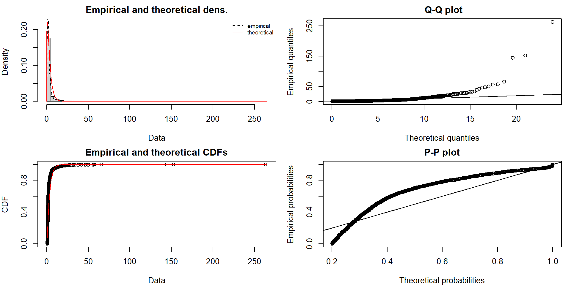
Context: Insurance companies model loss amounts using gamma distributions because losses are naturally right-skewed with a long tail of catastrophic events. We analyze Danish fire insurance losses from 1980-1990.

Key Questions:

What are the optimal shape ($\alpha$) and scale ($\beta$) parameters using MLE?
What proportion of losses exceed certain thresholds (e.g., 10M, 20M DKK)?
How well does the gamma model fit, and what are its limitations?

📊 Data Source

We analyze Danish fire insurance losses (1980-1990) - a classic actuarial dataset.

Source: R package fitdistrplus - danishuni dataset

Sample Size: 2,167 individual fire insurance claims

Data Type: Loss amounts in millions of Danish Krone (DKK)

Application: Widely used for demonstrating actuarial modeling, extreme value analysis, and heavy-tailed distributions

💰 Case Study: Data Loading and Parameter Estimation

Code

# Load required libraries
library(tidyverse)
library(fitdistrplus)  # For MLE fitting

# Load real insurance loss data from fitdistrplus package
# Danish fire insurance losses (1980-1990): 2,167 claims
# This is a classic actuarial dataset for gamma distribution modeling
data(danishuni)

# Extract loss amounts (in millions of Danish Krone)
claims <- danishuni$Loss

# Verify we have sufficient data
if (length(claims) < 100) {
  stop(paste("Error: Only", length(claims), "claims loaded. Need at least 100."))
}

cat("Data source: Danish fire insurance losses (1980-1990)\n")

Data source: Danish fire insurance losses (1980-1990)

Code

cat("Original values in millions of Danish Krone\n")

Original values in millions of Danish Krone

Code

# Summary statistics
n_claims <- length(claims)
mean_claim <- mean(claims)
median_claim <- median(claims)
sd_claim <- sd(claims)
max_claim <- max(claims)

cat(sprintf("Sample size: %d claims\n", n_claims))

Sample size: 2167 claims

Code

cat(sprintf("Mean claim: $%.2f\n", mean_claim))

Mean claim: $3.39

Code

cat(sprintf("Median claim: $%.2f\n", median_claim))

Median claim: $1.78

Code

cat(sprintf("Std Dev: $%.2f\n", sd_claim))

Std Dev: $8.51

Code

cat(sprintf("Max claim: $%.2f\n", max_claim))

Max claim: $263.25

Code

# Estimate gamma parameters using Maximum Likelihood Estimation (MLE)
# MLE provides optimal parameter estimates for the gamma distribution
# fitdistrplus uses numerical optimization for robust fitting

fit_gamma <- fitdist(claims, "gamma", method = "mle")

# Extract parameters (note: fitdist uses shape and rate parameterization)
alpha_est <- fit_gamma$estimate["shape"]
rate_est <- fit_gamma$estimate["rate"]
beta_est <- 1 / rate_est  # Convert rate to scale parameter

cat(sprintf("Shape (α): %.3f\n", alpha_est))

Shape (α): 1.298

Code

cat(sprintf("Scale (β): %.2f M DKK\n", beta_est))

Scale (β): 2.61 M DKK

Code

cat(sprintf("Rate (1/β): %.4f\n", rate_est))

Rate (1/β): 0.3833

Code

cat(sprintf("\nEstimated mean: %.2f M DKK\n", 
            alpha_est * beta_est))


Estimated mean: 3.39 M DKK

Code

cat(sprintf("Sample mean: %.2f M DKK\n", mean_claim))

Sample mean: 3.39 M DKK

Code

cat(sprintf("\nEstimated SD: %.2f M DKK\n", 
            sqrt(alpha_est * beta_est^2)))


Estimated SD: 2.97 M DKK

Code

cat(sprintf("Sample SD: %.2f M DKK\n", sd_claim))

Sample SD: 8.51 M DKK

Code

cat(sprintf("\nLog-likelihood: %.2f\n", fit_gamma$loglik))


Log-likelihood: -4767.10


Probabilities of Exceeding Thresholds

=====================================

P(Loss > 5M DKK): 0.2231 (22.31%)

P(Loss > 10M DKK): 0.0384 (3.84%)

P(Loss > 20M DKK): 0.0010 (0.10%)

💰 Case Study: Visualization and Model Validation

💰 Model Fit Assessment: Interpreting Diagnostic Plots

📊 Observations

From the diagnostic plots:

Histogram/Density: Overall fit appears reasonable for the bulk of the data
Q-Q Plot (Quantile-Quantile): Shows departure from the reference line in the upper tail (right side)
P-P Plot (Probability-Probability): Shows systematic deviation, especially in the tails

⚠️ Why the Departure?

Heavy-tailed nature: Fire insurance losses have heavier tails than the gamma distribution can capture
Extreme values: A few very large losses (>100M DKK) create tail behavior that deviates from gamma
Not a problem with estimation: MLE is correctly estimating gamma parameters, but gamma may not be the ideal model for extreme losses

💡 Better Alternatives

For heavy-tailed data:

Pareto distribution: Specifically designed for heavy tails
Log-normal distribution: Often fits insurance claims better
Generalized Pareto (GPD): Used in extreme value theory
Mixture models: Combine gamma for moderate losses + extreme value distribution for large losses

📚 Key Lesson

Gamma is useful for moderate right-skewed data, but real insurance losses often require more sophisticated models.

💰 Case Study: Actuarial Applications and Pricing

📊 Distributional Characteristics

Danish Fire Insurance Losses 1980-1990:

Shape parameter $\alpha \approx 1.30$: Indicates moderate right skew typical of insurance losses
Scale parameter $\beta \approx 2.61$ million DKK: Controls the spread of loss amounts
Mean loss: $\alpha \times \beta \approx 3.39$ million DKK per claim
Interpretation: $\alpha > 1$ means the distribution has a mode away from zero, with a substantial right tail for catastrophic losses

💼 Business Applications

Premium Pricing Strategy:

Pure premium = Expected loss cost = $\mu \approx 3.39$ million DKK per policy
Loading for risk: Add safety margin for tail losses using percentiles (e.g., 90th, 95th, 99th)
Risk assessment: Coefficient of variation $\text{CV} = 1/\sqrt{\alpha} \approx 0.88$ indicates moderate variability

Reserve Estimation: The gamma model with $\alpha \approx 1.3$ captures realistic fire insurance loss patterns: most claims are moderate, with a long tail for major fires requiring substantial reserves.

📝 Quiz #1: Gamma Distribution Parameters

For a gamma distribution with $\alpha = 3$ and $\beta = 5$, what is the mean?

$\mu = 15$
$\mu = 8$
$\mu = 75$
$\mu = 3$

📝 Quiz #2: Chi-Square Relationship

A random variable $Y$ has a gamma distribution with $\alpha = 4$ and $\beta = 2$. What distribution does $\frac{2Y}{\beta} = Y$ follow?

$\chi^2$ with 8 degrees of freedom
$\chi^2$ with 4 degrees of freedom
$\chi^2$ with 2 degrees of freedom
Exponential with parameter 2

📝 Quiz #3: Exponential Distribution

Which property uniquely characterizes the exponential distribution among continuous distributions?

The memoryless property: P(Y > a + b | Y > a) = P(Y > b)
It has mean equal to variance
It is symmetric around its mean
It has bounded support

📝 Quiz #4: Variance Formula

If a gamma-distributed random variable has $\alpha = 2$ and variance $\sigma^2 = 32$, what is the scale parameter $\beta$?

$\beta = 4$
$\beta = 16$
$\beta = 8$
$\beta = 2$

📝 Summary

✅ Key Takeaways

The gamma distribution is a flexible two-parameter family ($\alpha$ and $\beta$) that models right-skewed, non-negative continuous data such as waiting times, claim amounts, and component lifetimes
Special cases include the exponential distribution ($\alpha = 1$) and chi-square distribution ($\alpha = \nu/2$, $\beta = 2$), each with specific applications in reliability, queuing, and statistical inference
The exponential distribution possesses the unique memoryless property, making it suitable for modeling random arrivals and component failures where past history doesn’t affect future probabilities
Mean and variance formulas ($\mu = \alpha\beta$ and $\sigma^2 = \alpha\beta^2$) allow parameter estimation from sample data using method of moments or maximum likelihood
Financial applications include insurance loss modeling, credit risk assessment, reliability engineering, and income distribution analysis, where the gamma family captures realistic skewness and tail behavior

📚 Practice Problems

📝 Homework Problems

Problem 1 (Insurance Claims): An insurance company models claim amounts using a gamma distribution with mean $15,000 and variance $112,500,000. Find: (a) the parameters $\alpha$ and $\beta$; (b) the probability a claim exceeds $30,000; (c) the 95th percentile of claim amounts for reserve planning.

Problem 2 (System Reliability): The lifetime of a critical server component follows an exponential distribution with mean 5000 hours. (a) What is the probability the component fails before 3000 hours? (b) Given it has already operated for 2000 hours, what is the probability it operates for at least 4000 additional hours? (c) Compare this to a non-memoryless distribution’s behavior.

Problem 3 (Hypothesis Testing): In testing whether a sample variance differs from a population variance, we use the chi-square distribution. If a sample of size $n = 25$ has variance $s^2 = 36$ and we’re testing against a hypothesized $\sigma^2 = 25$, calculate the chi-square test statistic $\chi^2 = \frac{(n-1)s^2}{\sigma^2}$ and find the probability of observing a value this extreme or more.

Problem 4 (Water Resources): Daily water consumption in a district follows a gamma distribution with $\alpha = 3$ and $\beta = 200$ thousand gallons. What capacity should be maintained to ensure demand is met 99% of days?

👋 Thank You!

📬 Contact Information:

Samir Orujov, PhD

Assistant Professor

School of Business

ADA University

📧 Email: sorujov@ada.edu.az

🏢 Office: D312

⏰ Office Hours: By appointment

📅 Next Class:

Topic: Sampling Distributions and the Central Limit Theorem

Reading: Chapter 8 (textbook sections on sampling distributions)

Preparation: Review properties of sums of random variables and convolution

⏰ Reminders:

✅ Complete Practice Problems 1-4

✅ Explore online gamma/chi-square calculators

✅ Review integration by parts technique

✅ Work hard!

❓ Questions?

💬 Open Discussion (5 minutes)

Key Topics for Discussion:

How do insurance companies use gamma distributions to set premiums that balance competitiveness with profitability and solvency requirements?
What are the limitations of the memoryless property assumption in financial modeling, and when might alternative distributions (Weibull, log-normal) be more appropriate?
How does the chi-square distribution connect to hypothesis testing for variance and goodness-of-fit tests in econometrics?
In reliability engineering, how do gamma distributions with different shape parameters model different failure mechanisms (wear-out vs. random failure)?

Mathematical Statistics

🎯 Learning Objectives

📋 Overview

📖 Definition: Skewed Distribution

📊 Types of Skewness

📌 Example 1: Human Lifespan Distribution

📖 Definition: Gamma Probability Distribution

🔍 Understanding Gamma Parameters

🧮 Theorem: Mean and Variance of Gamma Distribution

🎮 Interactive: Gamma Distribution Explorer

📌 Example 2: Computer Response Time

📌 Example 2: Solution (continued)

📌 Example 2: Integration by Parts

🤝 Think-Pair-Share: IT Infrastructure Planning

📖 Definition: Chi-Square Distribution

🔗 Relationship: Gamma to Chi-Square

📌 Example 3: Converting Gamma to Chi-Square

🎮 Interactive: Chi-Square Distribution by Degrees of Freedom

📖 Definition: Exponential Distribution

🔍 The Memoryless Property

📌 Example 4: Memoryless Property Verification

📌 Example 4: Solution (continued)

🎮 Interactive: Exponential Distribution

📌 Example 5: Water Demand at Pumping Station

📌 Example 5: Solution (continued)

📌 Example 5: Solution (continued)

💰 Case Study: Insurance Claim Amounts (Real Data)

💰 Case Study: Data Loading and Parameter Estimation

💰 Case Study: Visualization and Model Validation

💰 Model Fit Assessment: Interpreting Diagnostic Plots

💰 Case Study: Actuarial Applications and Pricing

📝 Quiz #1: Gamma Distribution Parameters

📝 Quiz #2: Chi-Square Relationship

📝 Quiz #3: Exponential Distribution

📝 Quiz #4: Variance Formula

📝 Summary

📚 Practice Problems

👋 Thank You!

❓ Questions?