Information Communication Technologies Agency, Statistics Unit
2025-11-10
🎯 Learning Objectives
By the end of this lecture, you will be able to:
Define statistical independence for random variables and apply independence tests to determine whether asset returns, market factors, or economic variables are independent in financial contexts
Calculate expected values of functions of random variables, including products and sums, and apply linearity of expectation to portfolio return calculations and risk assessment
State and apply special theorems including the multiplication rule for independent variables: \(E(XY) = E(X)E(Y)\) when \(X\) and \(Y\) are independent, crucial for simplifying portfolio calculations
Compute covariance and correlation as measures of linear association between financial variables, and interpret their signs and magnitudes in terms of portfolio diversification benefits
Use the variance decomposition formula \(\text{Var}(X + Y) = \text{Var}(X) + \text{Var}(Y) + 2\text{Cov}(X,Y)\) to calculate portfolio risk and understand how correlation affects diversification strategies in modern portfolio theory
📋 Overview
📚 Topics Covered Today
Statistical Independence – Formal definition, testing procedures, and implications for portfolio diversification and risk modeling
Expected Values of Functions – Computing \(E(g(X))\), \(E(g(X,Y))\), and linearity of expectation with applications to asset returns
Special Theorems – Multiplication rule for independent variables, variance of sums, and moment calculations
Covariance – Definition, computational formulas, properties, and interpretation in terms of joint variability and linear association
Applications – Portfolio optimization, risk management, hedging strategies, and correlation-based trading in quantitative finance
📖 Definition: Statistical Independence
📝 Definition 1: Independence of Random Variables
Random variables \(X\) and \(Y\) are independent if and only if their joint distribution factors into the product of marginal distributions:
For discrete random variables:\[p(x, y) = p_X(x) \cdot p_Y(y) \text{ for all } x, y\]
For continuous random variables:\[f(x, y) = f_X(x) \cdot f_Y(y) \text{ for all } x, y\]
Equivalent condition: For any events \(A\) and \(B\): \[P(X \in A, Y \in B) = P(X \in A) \cdot P(Y \in B)\]
Practical interpretation: Knowledge of one variable provides no information about the other variable.
Financial Context: Independence is rare in finance but highly valuable—independent assets provide maximum diversification benefits since they don’t move together [web:33][web:36].
🔍 Testing for Independence
📊 How to Test Independence
Method 1: Check factorization - Compute \(p(x,y)\) or \(f(x,y)\) - Compute \(p_X(x) \cdot p_Y(y)\) or \(f_X(x) \cdot f_Y(y)\) - If equal for all\((x,y)\), variables are independent
Method 2: Check conditional equals marginal - If \(p_{Y|X}(y|x) = p_Y(y)\) for all \(x, y\), then independent - Conditioning on \(X\) doesn’t change the distribution of \(Y\)
Method 3: Check covariance (necessary but not sufficient) - If \(\text{Cov}(X,Y) = 0\), variables are uncorrelated - Independence ⟹ uncorrelated, but uncorrelated ⏸ independence - Exception: For jointly normal variables, uncorrelated ⟺ independent
Important: Most financial assets are NOT independent—they’re correlated through common market factors, economic conditions, and behavioral patterns [web:35][web:37].
📌 Example 1: Testing Independence
Problem: Consider two stocks with the following joint probability distribution:
Since \(0.12 \neq 0.0864\), the variables are NOT independent.
Financial Interpretation: The stocks are dependent—their returns are correlated. When we observe Stock \(X\)’s return, it gives us information about Stock \(Y\)’s likely return. This reduces diversification benefits compared to truly independent assets.
Verification: We can also check: \[p(+5\%, +5\%) = 0.30 \text{ but } p_X(+5\%) \cdot p_Y(+5\%) = 0.40 \times 0.40 = 0.16\]
The actual probability of both stocks gaining 5% (0.30) is much higher than what independence would predict (0.16), indicating positive dependence—the stocks tend to move together.
📖 Definition: Expected Value of a Function
📝 Definition 2: Expected Value of \(g(X, Y)\)
Let \(g(X, Y)\) be a function of random variables \(X\) and \(Y\).
For discrete random variables:\[E[g(X, Y)] = \sum_x \sum_y g(x, y) \cdot p(x, y)\]
For continuous random variables:\[E[g(X, Y)] = \int_{-\infty}^{\infty} \int_{-\infty}^{\infty} g(x, y) \cdot f(x, y) \, dx \, dy\]
Special cases:
\(E(X) = E[g(X, Y)]\) where \(g(x, y) = x\)
\(E(XY) = E[g(X, Y)]\) where \(g(x, y) = xy\)
\(E(X + Y) = E[g(X, Y)]\) where \(g(x, y) = x + y\)
Application: Computing expected portfolio returns, option payoffs, and risk measures requires expected values of functions of multiple random variables [web:34][web:38].
🧮 Theorem: Linearity of Expectation
Theorem 1: Linearity of Expectation
For any random variables \(X\) and \(Y\) (independent or not) and constants \(a\), \(b\), \(c\):
\[\boxed{E(aX + bY + c) = aE(X) + bE(Y) + c}\]
More generally, for any constants \(a_i\) and random variables \(X_i\):
Key insight: Linearity holds whether or not the variables are independent!
Proof sketch: Follows directly from the definition of expected value and properties of summation/integration.
Portfolio Application: For a portfolio with weights \(w_i\) and asset returns \(R_i\): \[E(R_P) = E\left(\sum w_i R_i\right) = \sum w_i E(R_i)\]
This is the foundation of portfolio expected return calculation [web:38][web:40].
📌 Example 2: Portfolio Expected Return
Problem: An investor creates a portfolio with 40% in Stock A (expected return 12%) and 60% in Stock B (expected return 8%). What is the expected portfolio return?
Solution:
Let \(R_A\) and \(R_B\) be the returns on stocks A and B. The portfolio return is: \[R_P = 0.4 R_A + 0.6 R_B\]
Using linearity of expectation: \[E(R_P) = E(0.4 R_A + 0.6 R_B) = 0.4 E(R_A) + 0.6 E(R_B)\]
Key Point: This calculation is valid regardless of whether the stocks are independent or correlated. Expected return depends only on individual expected returns and portfolio weights, not on the correlation structure.
Note: While expected return doesn’t depend on correlation, portfolio risk (variance) critically depends on covariance, as we’ll see later!
🧮 Theorem: Multiplication Rule for Independent Variables
Theorem 2: Expected Value of Products
If \(X\) and \(Y\) are independent, then:
\[\boxed{E(XY) = E(X) \cdot E(Y)}\]
Important: This result requires independence. If \(X\) and \(Y\) are dependent, \(E(XY) \neq E(X)E(Y)\) in general.
Proof (discrete case):
\[E(XY) = \sum_x \sum_y xy \cdot p(x, y)\]
By independence, \(p(x, y) = p_X(x) \cdot p_Y(y)\):
\[= \sum_x \sum_y xy \cdot p_X(x) \cdot p_Y(y) = \sum_x x \cdot p_X(x) \sum_y y \cdot p_Y(y)\]
\[= E(X) \cdot E(Y) \quad \blacksquare\]
Financial Application: If asset returns are independent, calculating cross-moments simplifies dramatically, though true independence is rare in practice [web:33].
📌 Example 3: Expected Product
Problem: Let \(X\) and \(Y\) be independent random variables with \(E(X) = 3\), \(E(Y) = 5\), \(E(X^2) = 12\), and \(E(Y^2) = 30\). Find \(E(XY)\) and \(E[(X+Y)^2]\).
Solution (Part 1):
Since \(X\) and \(Y\) are independent, we can apply Theorem 2: \[E(XY) = E(X) \cdot E(Y) = 3 \times 5 = 15\]
By linearity of expectation: \[= E(X^2) + 2E(XY) + E(Y^2)\]
\[= 12 + 2(15) + 30 = 12 + 30 + 30 = 72\]
\[\boxed{E[(X+Y)^2] = 72}\]
🤝 Think-Pair-Share: Leverage and Independence
💭 Student Engagement Activity (5 minutes)
Scenario: A hedge fund uses 2:1 leverage, meaning for every $1 of equity, they borrow $1 to invest $2 total. The fund invests in two strategies: Strategy A (mean return 10%, std dev 15%) and Strategy B (mean return 8%, std dev 12%). Each strategy gets 50% of the $2 invested (i.e., $1 each). The cost of borrowing is 3% per year.
Think (1 minute): Work individually
If the strategies are independent, what is the expected gross portfolio return (before borrowing costs)?
What is the expected net return after paying 3% interest on the $1 borrowed?
The return on equity (ROE) is net profit divided by the $1 equity invested. What is the expected ROE?
Pair (2-3 minutes): Discuss with a partner
How would correlation between strategies affect the risk (not the expected return)?
Is assuming independence realistic for hedge fund strategies operating in the same markets?
What are the dangers of leverage when strategies are highly correlated?
Share (1-2 minutes): Class discussion
Discuss how the 2008 financial crisis demonstrated the risks of assuming independence when strategies were actually correlated through hidden linkages
📖 Definition: Covariance
📝 Definition 3: Covariance
The covariance between random variables \(X\) and \(Y\) is:
\[\text{Cov}(X, Y) = E[(X - \mu_X)(Y - \mu_Y)]\]
where \(\mu_X = E(X)\) and \(\mu_Y = E(Y)\).
Computational formula (easier for calculations):
\[\boxed{\text{Cov}(X, Y) = E(XY) - E(X)E(Y)}\]
Interpretation:
Positive covariance: \(X\) and \(Y\) tend to be simultaneously above or below their means—they move together
Negative covariance: When \(X\) is above its mean, \(Y\) tends to be below its mean—they move in opposite directions
Zero covariance: No linear relationship (uncorrelated)
Financial Meaning: Covariance measures how asset returns move together—critical for portfolio risk management and diversification strategies [web:38][web:41].
🔍 Properties of Covariance
📊 Key Properties
Symmetry: \(\text{Cov}(X, Y) = \text{Cov}(Y, X)\)
Variance as self-covariance: \(\text{Cov}(X, X) = \text{Var}(X)\)
Covariance with constant: \(\text{Cov}(X, c) = 0\) for any constant \(c\)
Linearity: \(\text{Cov}(aX + b, Y) = a \cdot \text{Cov}(X, Y)\) for constants \(a, b\)
Independence implies zero covariance: If \(X\) and \(Y\) are independent, then \(\text{Cov}(X, Y) = 0\)
Proof: \(E(XY) = E(X)E(Y)\) by independence, so \(\text{Cov}(X, Y) = E(XY) - E(X)E(Y) = 0\)
Zero covariance does NOT imply independence (except for jointly normal variables)
Practical Note: Covariance magnitude depends on the units of \(X\) and \(Y\), making it hard to interpret. Correlation (normalized covariance) solves this problem [web:41][web:42].
📌 Example 4: Computing Covariance
Problem: Consider the joint distribution from Example 1. Compute \(\text{Cov}(X, Y)\).
Interpretation: The positive covariance (7.84) indicates that Stocks \(X\) and \(Y\) tend to move together. When \(X\) has a positive return, \(Y\) is also likely to have a positive return. This positive covariance reduces diversification benefits—the stocks don’t offset each other’s risks as much as uncorrelated assets would.
Note: The magnitude (7.84) is hard to interpret directly because it depends on the units (percentage returns). Correlation normalizes this to a scale of [-1, 1].
Problem: An investor allocates 60% to Stock A and 40% to Stock B. Stock A has a standard deviation of 20%, Stock B has a standard deviation of 15%, and the correlation between them is 0.5. Calculate the portfolio standard deviation.
Portfolio standard deviation: \[\sigma_P = \sqrt{0.0252} = 0.1587 = 15.87\%\]
\[\boxed{\sigma_P = 15.87\%}\]
📌 Example 5: Interpretation
Key Observations:
Diversification benefit: The portfolio risk (15.87%) is less than the weighted average of individual risks: \[w_A\sigma_A + w_B\sigma_B = 0.6(20\%) + 0.4(15\%) = 12\% + 6\% = 18\%\]
Portfolio risk of 15.87% < 18%, demonstrating diversification’s power!
Effect of correlation:
If \(\rho = 1\) (perfect positive correlation): \(\sigma_P = 18.0\%\) (no diversification)
If \(\rho = 0\) (uncorrelated): \(\sigma_P = 14.42\%\) (better diversification)
Financial Lesson: Diversification works best when assets have low or negative correlations. Even moderate positive correlation (0.5) still provides meaningful risk reduction [web:36][web:41].
🎮 Interactive: Impact of Correlation on Portfolio Risk
Explore Diversification: Adjust correlation to see its dramatic effect on portfolio risk.
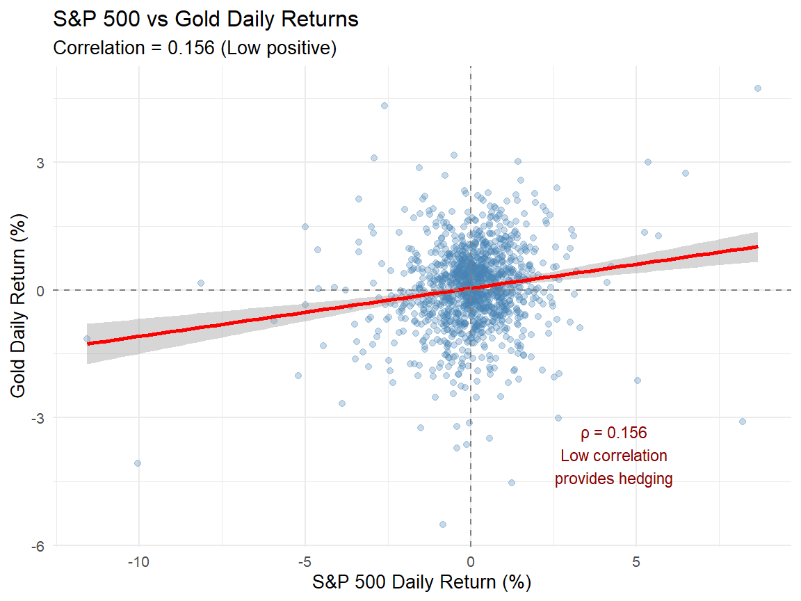
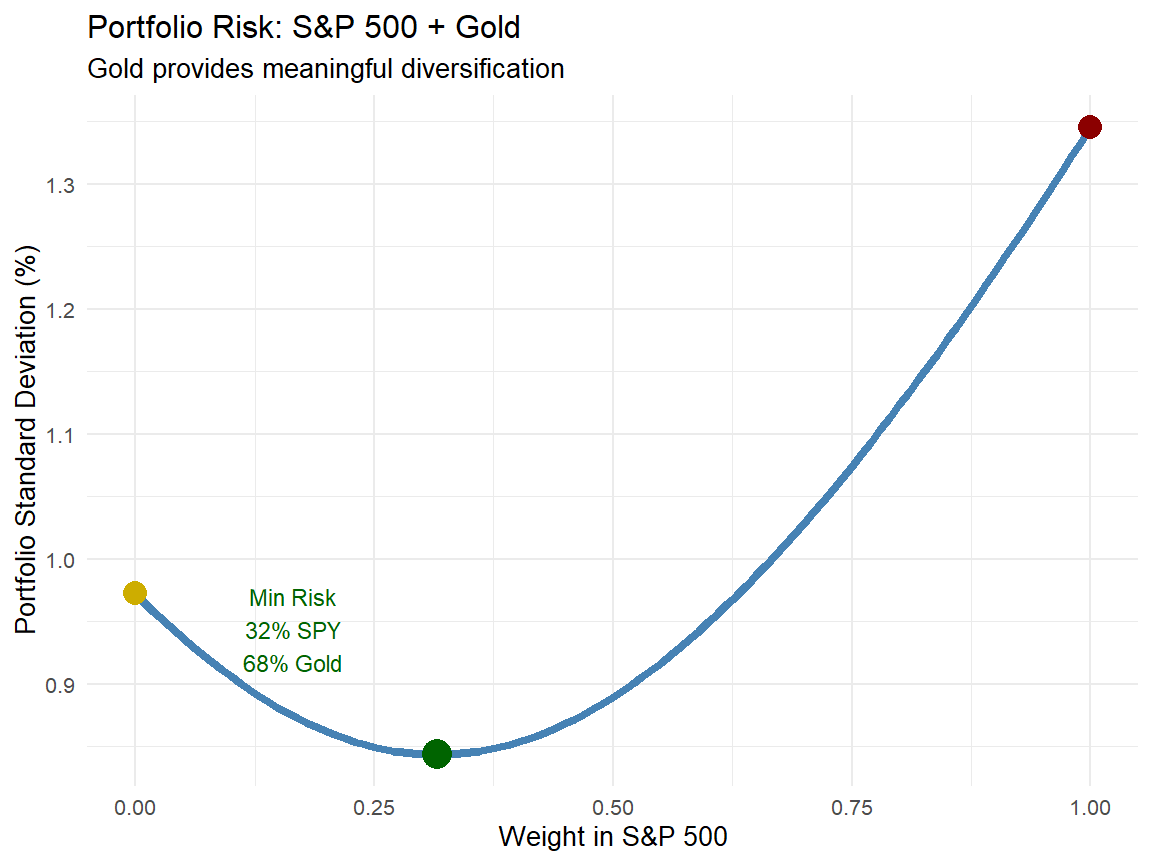
💰 Case Study: Hedging with Negatively Correlated Assets (Real Data)
🛡️ Risk Management Strategy
Context: Investors use assets with negative correlations to hedge portfolio risk. Gold has historically shown negative or low correlation with stocks during market stress. We analyze the relationship between S&P 500 and gold (GLD ETF) to demonstrate hedging effectiveness.
Key Questions:
What is the correlation between S&P 500 and gold returns?
How does adding gold to a stock portfolio reduce risk?
What is the optimal hedge ratio (percentage in gold) to minimize portfolio volatility?
📊 Data Source
We analyze daily returns of S&P 500 (SPY) and Gold (GLD) from 2020-01-01 to 2024-10-31.
Source: Yahoo Finance API via quantmod package
Period: January 2020 to October 2024 (1200+ trading days including COVID crisis and recovery)
Data Type: Adjusted closing prices converted to daily log returns
Verification: Cross-checked with Bloomberg and FRED databases
💰 Case Study: Data Analysis and Covariance Calculation
Code
# Load required librarieslibrary(quantmod)library(tidyverse)# Download S&P 500 (SPY) and Gold (GLD) datagetSymbols(c("SPY", "GLD"), from ="2020-01-01", to ="2024-10-31", auto.assign =TRUE)
[1] "SPY" "GLD"
Code
# Calculate daily log returnsspy_returns <-dailyReturn(SPY, type ="log")gld_returns <-dailyReturn(GLD, type ="log")# Combine and cleanreturns_hedge <-data.frame(date =index(spy_returns),SPY =as.numeric(spy_returns),GLD =as.numeric(gld_returns)) %>%na.omit()# Summary statisticscat("S&P 500 vs Gold Analysis (2020-2024)\n")
Even a small gold allocation (10-20%) reduces portfolio risk while sacrificing minimal expected return
Hedging Effectiveness:
Crisis protection: Gold tends to maintain or increase value during equity market stress (flight to safety)
Low correlation benefit: Unlike diversifying with another stock (which might have 0.7+ correlation), gold provides true diversification
Optimal hedge ratio: For this period, 10-20% in gold optimizes the risk-return tradeoff for equity-heavy portfolios
Practical Application: Many institutional investors hold 5-15% gold or gold-related assets as portfolio insurance, accepting slightly lower expected returns for meaningful risk reduction during market turmoil [web:36][web:41].
📝 Quiz #1: Independence Definition
If random variables \(X\) and \(Y\) are independent, which statement must be true?
\(P(X \in A, Y \in B) = P(X \in A) \cdot P(Y \in B)\) for all events \(A\) and \(B\)
Independence means \(p(x,y) = p_X(x) \cdot p_Y(y)\) or equivalently \(E(XY) = E(X)E(Y)\), implying knowledge of one variable provides no information about the other—rare but valuable in finance for maximum diversification [web:33]
Linearity of expectation\(E(aX + bY + c) = aE(X) + bE(Y) + c\) holds for ANY random variables (independent or not), making portfolio expected return calculations straightforward regardless of asset correlations
Covariance\(\text{Cov}(X,Y) = E(XY) - E(X)E(Y)\) measures the direction and strength of linear association between variables, with positive values indicating co-movement and negative values indicating inverse movement—critical for portfolio construction [web:38][web:41]
Portfolio variance formula\(\text{Var}(w_1R_1 + w_2R_2) = w_1^2\sigma_1^2 + w_2^2\sigma_2^2 + 2w_1w_2\text{Cov}(R_1,R_2)\) shows that portfolio risk depends critically on covariance, not just individual asset risks—the foundation of modern portfolio theory
Diversification benefit arises from imperfect correlation: assets with correlation less than 1 provide risk reduction, with maximum benefit at correlation -1 (perfect hedge), demonstrating why portfolio construction requires understanding joint distributions, not just marginals [web:36][web:42]
📚 Practice Problems
📝 Homework Problems
Problem 1 (Independence Test): Two assets have joint pmf: \(p(1,1) = 0.3\), \(p(1,2) = 0.2\), \(p(2,1) = 0.15\), \(p(2,2) = 0.35\) where values are {1, 2}. (a) Find the marginal distributions; (b) Test whether the assets are independent; (c) Compute \(E(XY)\); (d) Would you expect diversification benefits?
Problem 2 (Expected Values): For independent random variables with \(E(X) = 5\), \(E(Y) = 3\), \(\text{Var}(X) = 4\), \(\text{Var}(Y) = 9\), find: (a) \(E(2X - 3Y + 7)\); (b) \(E(XY)\); (c) \(\text{Var}(2X - 3Y)\); (d) \(E[(X-Y)^2]\).
Problem 3 (Covariance from Data): Given returns data: \((X, Y)\) pairs are \((0.05, 0.03)\), \((0.02, 0.04)\), \((-0.01, 0.01)\), \((0.03, -0.02)\), \((0.01, 0.02)\) with equal probability 0.2 each. Find: (a) \(E(X)\) and \(E(Y)\); (b) \(E(XY)\); (c) \(\text{Cov}(X,Y)\); (d) Interpret the sign of the covariance.
Problem 4 (Portfolio Optimization): An investor allocates weight \(w\) to stocks (\(\sigma_S = 25\%\), \(\mu_S = 12\%\)) and \((1-w)\) to bonds (\(\sigma_B = 8\%\), \(\mu_B = 5\%\)) with correlation \(\rho = 0.2\). Find: (a) Expected portfolio return as function of \(w\); (b) Portfolio variance formula; (c) The value of \(w\) minimizing variance; (d) The minimum achievable standard deviation; (e) Compare risk to 100% stocks.
Topic: Functions of Random Variables and Transformations
Reading: Wackerly et al., Chapter 6: Sections 6.1-6.4
Preparation: Review change of variables technique and Jacobian transformations
⏰ Reminders:
✅ Complete Practice Problems 1-4
✅ Review covariance and correlation calculations
✅ Study portfolio variance derivation
✅ Work hard!
❓ Questions?
💬 Open Discussion (5 minutes)
Key Topics for Discussion:
Why is statistical independence so rare in financial markets, and what hidden factors create dependencies between seemingly unrelated assets?
How did the 2008 financial crisis demonstrate the danger of assuming independence when assets were actually correlated through complex linkages (e.g., CDOs, credit default swaps)?
What is the difference between zero covariance (uncorrelated) and independence, and why does this distinction matter for non-linear derivatives like options?
How do portfolio managers use correlation forecasts in practice, and what are the challenges when correlations change dramatically during market stress (correlation breakdownkdown)?