Mathematical Statistics

🎯 Learning Objectives

By the end of this lecture, you will be able to:

Define bivariate and multivariate probability distributions and compute joint, marginal, and conditional probabilities for discrete and continuous random variables
Calculate and interpret covariance and correlation coefficients as measures of linear association between financial assets, and understand their role in portfolio risk management
Apply the concept of conditional distributions to model dependencies between variables and compute conditional expectations in financial contexts (e.g., option pricing, credit risk)
Determine whether random variables are independent using joint and marginal distributions, and understand the implications for portfolio diversification
Construct optimal financial portfolios using bivariate distributions to balance expected return and risk through proper understanding of asset correlations and covariances

📋 Overview

📚 Topics Covered Today

Joint Probability Distributions – Bivariate discrete and continuous distributions modeling multiple random variables simultaneously
Marginal Distributions – Extracting individual variable distributions from joint distributions by summation or integration
Conditional Distributions – Modeling one variable given knowledge of another, essential for risk assessment and forecasting
Covariance and Correlation – Measuring linear association between variables, fundamental to modern portfolio theory
Independence – Testing statistical independence and understanding diversification benefits in investment portfolios

📖 Definition: Joint Probability Distribution

📝 Definition 1: Bivariate Discrete Distribution

Let $X$ and $Y$ be two discrete random variables. The joint probability mass function (pmf) $p(x, y)$ is:

\[p(x, y) = P(X = x, Y = y)\]

for all pairs $(x, y)$ in the sample space.

Properties:

Non-negativity: $p(x, y) \geq 0$ for all $(x, y)$
Total probability: $\sum_x \sum_y p(x, y) = 1$ (sum over all possible values)
Event probabilities: For any region $A$ in the sample space, $P((X, Y) \in A) = \sum_{(x,y) \in A} p(x, y)$

Financial Context: Joint distributions model relationships between multiple assets (e.g., stock returns of two companies), interest rate movements and inflation, or trading volume and price changes [web:23][web:28].

📌 Example 1: Joint Distribution of Two Stocks

Problem: A financial analyst models the daily returns of two technology stocks, $X$ (Stock A) and $Y$ (Stock B). The joint probability distribution is given in the table below:

	$Y = -1\%$	$Y = 0\%$	$Y = +1\%$
$X = -1\%$	0.10	0.05	0.05
$X = 0\%$	0.15	0.20	0.10
$X = +2\%$	0.05	0.10	0.20

Verify that this is a valid joint probability distribution.
Find $P(X = +2\%, Y = +1\%)$.
Find $P(X \geq 0\%)$.

Solution (Part a):

Check that all probabilities are non-negative: ✓ (all entries $\geq 0$)

Check that the sum equals 1: \[\sum_x \sum_y p(x, y) = 0.10 + 0.05 + \cdots + 0.20 = 1.00 \quad \checkmark\]

📌 Example 1: Solution (continued)

Solution (Part b):

From the table, we directly read: \[\boxed{P(X = +2\%, Y = +1\%) = 0.20}\]

Interpretation: There’s a 20% chance that both stocks will have their best outcomes simultaneously (Stock A gains 2% and Stock B gains 1%).

Solution (Part c):

\[P(X \geq 0\%) = P(X = 0\% \text{ or } X = +2\%)\]

Sum all probabilities in the bottom two rows: \[P(X = 0\%) = 0.15 + 0.20 + 0.10 = 0.45\] \[P(X = +2\%) = 0.05 + 0.10 + 0.20 = 0.35\] \[\boxed{P(X \geq 0\%) = 0.45 + 0.35 = 0.80}\]

Financial Insight: Stock A has an 80% probability of non-negative returns, suggesting it’s relatively stable or has a positive expected drift.

📖 Definition: Marginal Probability Distribution

📝 Definition 2: Marginal Distributions

Given a joint pmf $p(x, y)$, the marginal probability mass functions are obtained by summing over all values of the other variable:

Marginal distribution of $X$: \[p_X(x) = \sum_y p(x, y)\]

Marginal distribution of $Y$: \[p_Y(y) = \sum_x p(x, y)\]

Interpretation: The marginal distribution gives the probability distribution of one variable without regard to (or ignoring) the value of the other variable.

Financial Application: If we have a joint distribution of stock returns for two companies, the marginal distribution of one stock gives its individual return distribution regardless of the other stock’s performance [web:31].

📌 Example 2: Marginal Distributions from Example 1

Problem: Find the marginal distributions $p_X(x)$ and $p_Y(y)$ for the stock returns in Example 1.

Solution:

Marginal distribution of $X$ (Stock A):

\[p_X(-1\%) = 0.10 + 0.05 + 0.05 = 0.20\] \[p_X(0\%) = 0.15 + 0.20 + 0.10 = 0.45\] \[p_X(+2\%) = 0.05 + 0.10 + 0.20 = 0.35\]

Marginal distribution of $Y$ (Stock B):

\[p_Y(-1\%) = 0.10 + 0.15 + 0.05 = 0.30\] \[p_Y(0\%) = 0.05 + 0.20 + 0.10 = 0.35\] \[p_Y(+1\%) = 0.05 + 0.10 + 0.20 = 0.35\]

📌 Example 2: Interpretation

Stock A Marginal Distribution:

$x$	$p_X(x)$
$-1\%$	0.20
$0\%$	0.45
$+2\%$	0.35

Expected Return: \[E(X) = (-1)(0.20) + (0)(0.45) + (2)(0.35) = 0.50\%\]

Stock B Marginal Distribution:

$y$	$p_Y(y)$
$-1\%$	0.30
$0\%$	0.35
$+1\%$	0.35

Expected Return: \[E(Y) = (-1)(0.30) + (0)(0.35) + (1)(0.35) = 0.05\%\]

Key Insight: Stock A has higher expected return (0.50% vs 0.05%) but also potentially higher risk. The marginal distributions allow us to analyze each stock independently before considering portfolio effects.

🎮 Interactive: Joint and Marginal Distributions

Explore Joint Distributions: Adjust probabilities to see how joint distribution affects marginals.

📖 Definition: Conditional Probability Distribution

📝 Definition 3: Conditional Distributions

The conditional probability mass function of $Y$ given $X = x$ is:

\[p_{Y|X}(y|x) = P(Y = y \mid X = x) = \frac{p(x, y)}{p_X(x)}\]

provided $p_X(x) > 0$.

Similarly, the conditional pmf of $X$ given $Y = y$ is:

\[p_{X|Y}(x|y) = P(X = x \mid Y = y) = \frac{p(x, y)}{p_Y(y)}\]

provided $p_Y(y) > 0$.

Interpretation: Conditional distributions describe the probability distribution of one variable when we know the value of the other variable.

Financial Application: Given that the market declined today (conditioning event), what is the probability distribution of an individual stock’s return? This is critical for risk management and hedging strategies [web:25][web:31].

📌 Example 3: Conditional Distribution

Problem: Using the stock return data from Example 1, find the conditional distribution of $Y$ (Stock B) given that $X = +2\%$ (Stock A had a strong gain).

Solution:

First, recall the marginal probability: $p_X(+2\%) = 0.35$

From the joint distribution when $X = +2\%$: - $p(+2\%, -1\%) = 0.05$ - $p(+2\%, 0\%) = 0.10$ - $p(+2\%, +1\%) = 0.20$

Now compute the conditional probabilities:

\[p_{Y|X}(-1\% \mid +2\%) = \frac{0.05}{0.35} = \frac{1}{7} \approx 0.143\]

\[p_{Y|X}(0\% \mid +2\%) = \frac{0.10}{0.35} = \frac{2}{7} \approx 0.286\]

\[p_{Y|X}(+1\% \mid +2\%) = \frac{0.20}{0.35} = \frac{4}{7} \approx 0.571\]

📌 Example 3: Interpretation

Unconditional Distribution of $Y$:

$y$	$p_Y(y)$
$-1\%$	0.30
$0\%$	0.35
$+1\%$	0.35

Fairly balanced distribution

Conditional Distribution ($Y \mid X = +2\%$):

$y$	$p_{Y\mid X}(y \mid +2\%)$
$-1\%$	0.143
$0\%$	0.286
$+1\%$	0.571

Shifted toward positive returns!

Key Financial Insight: When Stock A performs very well (+2%), Stock B is much more likely to also perform well (+1% with 57% probability vs. 35% unconditionally). This suggests positive correlation between the stocks—they tend to move together. This has important implications for portfolio diversification: these two stocks do not provide strong diversification benefits since they’re positively correlated.

Conditional Expected Return: \[E(Y \mid X = +2\%) = (-1)(0.143) + (0)(0.286) + (1)(0.571) = 0.428\%\]

Much higher than the unconditional expected return of $E(Y) = 0.05\%$!

🤝 Think-Pair-Share: Portfolio Construction

💭 Student Engagement Activity (5 minutes)

Scenario: You are managing a $1,000,000 portfolio and considering two stocks with the joint distribution from Example 1. Stock A has $E(X) = 0.50\%$ daily return and Stock B has $E(Y) = 0.05\%$ daily return. You notice that when Stock A drops (-1%), Stock B’s conditional distribution becomes more favorable.

Think (1 minute): Work individually

Calculate the conditional expected return $E(Y \mid X = -1\%)$ using the joint distribution
Compare it to the unconditional $E(Y) = 0.05\%$
Does this suggest positive or negative correlation between the stocks?

Pair (2-3 minutes): Discuss with a partner

If the stocks were negatively correlated (one tends to rise when the other falls), how would this affect portfolio risk?
Would you invest 100% in Stock A (higher expected return) or create a diversified portfolio? Why?

Share (1-2 minutes): Class discussion

Discuss the trade-off between expected return and risk reduction through diversification
How does understanding conditional distributions help in making better portfolio decisions?

📖 Definition: Continuous Joint Distribution

📝 Definition 4: Bivariate Continuous Distribution

Let $X$ and $Y$ be continuous random variables. The joint probability density function (pdf) $f(x, y)$ satisfies:

\[P((X, Y) \in A) = \int \int_A f(x, y) \, dx \, dy\]

Properties:

Non-negativity: $f(x, y) \geq 0$ for all $(x, y)$
Total probability: $\int_{-\infty}^{\infty} \int_{-\infty}^{\infty} f(x, y) \, dx \, dy = 1$
Marginal densities: $f_X(x) = \int_{-\infty}^{\infty} f(x, y) \, dy$ and $f_Y(y) = \int_{-\infty}^{\infty} f(x, y) \, dx$
Conditional densities: $f_{Y|X}(y|x) = \frac{f(x, y)}{f_X(x)}$ for $f_X(x) > 0$

Application: Continuous joint distributions model asset returns, interest rates, volatilities, and other financial variables that can take any value in a continuous range [web:23].

📌 Example 4: Continuous Joint Distribution

Problem: Suppose the joint pdf of $(X, Y)$ is:

\[f(x, y) = \begin{cases} 2, & 0 \leq x \leq y \leq 1 \\ 0, & \text{elsewhere} \end{cases}\]

Verify this is a valid pdf.
Find the marginal density $f_X(x)$.
Find $P(X + Y \leq 1)$.

Solution (Part a):

Check non-negativity: ✓ ($f(x, y) \geq 0$ everywhere)

Check total probability equals 1: \[\int_{-\infty}^{\infty} \int_{-\infty}^{\infty} f(x, y) \, dy \, dx = \int_0^1 \int_x^1 2 \, dy \, dx\]

\[= \int_0^1 2[y]_x^1 \, dx = \int_0^1 2(1 - x) \, dx = 2\left[x - \frac{x^2}{2}\right]_0^1 = 2\left(1 - \frac{1}{2}\right) = 1 \quad \checkmark\]

📌 Example 4: Solution (continued)

Solution (Part b):

The marginal density of $X$ is: \[f_X(x) = \int_{-\infty}^{\infty} f(x, y) \, dy\]

Given the support $0 \leq x \leq y \leq 1$, for a fixed $x$, $y$ ranges from $x$ to $1$:

\[f_X(x) = \int_x^1 2 \, dy = 2[y]_x^1 = 2(1 - x), \quad 0 \leq x \leq 1\]

\[\boxed{f_X(x) = \begin{cases} 2(1 - x), & 0 \leq x \leq 1 \\ 0, & \text{elsewhere} \end{cases}}\]

Solution (Part c):

Find $P(X + Y \leq 1)$. The region is defined by $0 \leq x \leq y \leq 1$ and $x + y \leq 1$.

The constraint $x + y \leq 1$ combined with $y \geq x$ gives $y \leq 1 - x$.

Since we also need $y \geq x$, we require $x \leq 1 - x$, i.e., $x \leq 0.5$.

📌 Example 4: Solution (continued)

For $0 \leq x \leq 0.5$: $y$ ranges from $x$ to $1 - x$

\[P(X + Y \leq 1) = \int_0^{0.5} \int_x^{1-x} 2 \, dy \, dx\]

\[= \int_0^{0.5} 2[(1-x) - x] \, dx = \int_0^{0.5} 2(1 - 2x) \, dx\]

\[= 2\left[x - x^2\right]_0^{0.5} = 2\left(0.5 - 0.25\right) = 2(0.25) = 0.5\]

\[\boxed{P(X + Y \leq 1) = 0.5}\]

Interpretation: Half the probability mass lies in the region where $X + Y \leq 1$. If $X$ and $Y$ represented component lifetimes, this would indicate the probability that both fail before a combined time threshold.

📖 Definition: Independence

📝 Definition 5: Statistical Independence

Two random variables $X$ and $Y$ are independent if and only if:

For discrete random variables: \[p(x, y) = p_X(x) \cdot p_Y(y)\] for all pairs $(x, y)$.

For continuous random variables: \[f(x, y) = f_X(x) \cdot f_Y(y)\] for all pairs $(x, y)$.

Equivalent condition: $X$ and $Y$ are independent if and only if: \[P(X \in A, Y \in B) = P(X \in A) \cdot P(Y \in B)\] for all events $A$ and $B$.

Financial Interpretation: If two asset returns are independent, knowing one asset’s return provides no information about the other’s return. This is ideal for diversification—independent assets provide maximum risk reduction benefits [web:25].

📌 Example 5: Testing Independence

Problem: Are the stocks from Example 1 independent?

Solution:

Recall: $p_X(+2\%) = 0.35$ and $p_Y(+1\%) = 0.35$

If independent, we would have: \[p(+2\%, +1\%) \stackrel{?}{=} p_X(+2\%) \cdot p_Y(+1\%)\]

From the table: $p(+2\%, +1\%) = 0.20$

If independent: $p_X(+2\%) \cdot p_Y(+1\%) = 0.35 \times 0.35 = 0.1225$

Since $0.20 \neq 0.1225$, the stocks are NOT independent.

Financial Meaning: The stocks are dependent—their returns are correlated. When Stock A performs well, Stock B is more likely to also perform well than independence would predict (0.20 actual vs. 0.1225 expected under independence). This positive dependence reduces diversification benefits.

📖 Definition: Covariance

📝 Definition 6: Covariance

The covariance between random variables $X$ and $Y$ is:

\[\text{Cov}(X, Y) = E[(X - \mu_X)(Y - \mu_Y)]\]

where $\mu_X = E(X)$ and $\mu_Y = E(Y)$.

Computational formula: \[\boxed{\text{Cov}(X, Y) = E(XY) - E(X)E(Y)}\]

Properties:

If $X$ and $Y$ are independent, then $\text{Cov}(X, Y) = 0$ (converse not always true)
$\text{Cov}(X, X) = \text{Var}(X)$
$\text{Cov}(aX + b, cY + d) = ac \cdot \text{Cov}(X, Y)$ for constants $a, b, c, d$

Financial Interpretation: Positive covariance means assets tend to move together; negative covariance means they move in opposite directions—valuable for hedging [web:25][web:29].

🧮 Theorem: Variance of Sum of Random Variables

Theorem 1: Variance of Linear Combinations

For random variables $X$ and $Y$ and constants $a$ and $b$:

\[\boxed{\text{Var}(aX + bY) = a^2\text{Var}(X) + b^2\text{Var}(Y) + 2ab\text{Cov}(X, Y)}\]

Special case (portfolio of two assets with weights $w$ and $1-w$):

\[\text{Var}(wX + (1-w)Y) = w^2\sigma_X^2 + (1-w)^2\sigma_Y^2 + 2w(1-w)\text{Cov}(X, Y)\]

If $X$ and $Y$ are independent ($\text{Cov}(X, Y) = 0$):

\[\text{Var}(aX + bY) = a^2\text{Var}(X) + b^2\text{Var}(Y)\]

Critical Application: This formula is the foundation of modern portfolio theory and risk management. It shows that portfolio risk depends not only on individual asset risks but also on how assets co-move (covariance) [web:25][web:32].

📌 Example 6: Computing Covariance

Problem: For the stocks in Example 1, compute $\text{Cov}(X, Y)$.

Solution:

We already found: $E(X) = 0.50\%$ and $E(Y) = 0.05\%$

Now compute $E(XY)$: \[E(XY) = \sum_x \sum_y xy \cdot p(x, y)\]

\[= (-1)(-1)(0.10) + (-1)(0)(0.05) + (-1)(+1)(0.05)\] \[+ (0)(-1)(0.15) + (0)(0)(0.20) + (0)(+1)(0.10)\] \[+ (+2)(-1)(0.05) + (+2)(0)(0.10) + (+2)(+1)(0.20)\]

\[= 0.10 + 0 - 0.05 + 0 + 0 + 0 - 0.10 + 0 + 0.40 = 0.35\]

Using the computational formula: \[\text{Cov}(X, Y) = E(XY) - E(X)E(Y) = 0.35 - (0.50)(0.05)\]

\[\boxed{\text{Cov}(X, Y) = 0.35 - 0.025 = 0.325}\]

📖 Definition: Correlation Coefficient

📝 Definition 7: Correlation Coefficient

The correlation coefficient between $X$ and $Y$ is:

\[\boxed{\rho_{XY} = \text{Corr}(X, Y) = \frac{\text{Cov}(X, Y)}{\sigma_X \sigma_Y}}\]

where $\sigma_X = \sqrt{\text{Var}(X)}$ and $\sigma_Y = \sqrt{\text{Var}(Y)}$.

Properties:

$-1 \leq \rho_{XY} \leq 1$ (always bounded)
$\rho_{XY} = 1$: Perfect positive linear relationship
$\rho_{XY} = -1$: Perfect negative linear relationship
$\rho_{XY} = 0$: No linear relationship (uncorrelated)
Independent implies uncorrelated, but uncorrelated does not imply independent

Advantage over Covariance: Correlation is dimensionless and normalized, making it easy to interpret and compare across different asset pairs [web:29][web:32].

📌 Example 7: Computing Correlation

Problem: Find the correlation coefficient for the stocks in Example 1.

Solution:

First, compute the variances:

\[\text{Var}(X) = E(X^2) - [E(X)]^2\]

\[E(X^2) = (-1)^2(0.20) + (0)^2(0.45) + (2)^2(0.35) = 0.20 + 0 + 1.40 = 1.60\]

\[\text{Var}(X) = 1.60 - (0.50)^2 = 1.60 - 0.25 = 1.35\]

\[\sigma_X = \sqrt{1.35} \approx 1.162\]

Similarly: \[E(Y^2) = (-1)^2(0.30) + (0)^2(0.35) + (1)^2(0.35) = 0.30 + 0 + 0.35 = 0.65\]

\[\text{Var}(Y) = 0.65 - (0.05)^2 = 0.65 - 0.0025 = 0.6475\]

\[\sigma_Y = \sqrt{0.6475} \approx 0.805\]

📌 Example 7: Solution (continued)

Using $\text{Cov}(X, Y) = 0.325$ from Example 6:

\[\rho_{XY} = \frac{0.325}{(1.162)(0.805)} = \frac{0.325}{0.935} \approx 0.348\]

\[\boxed{\rho_{XY} \approx 0.348}\]

Financial Interpretation:

The correlation of 0.348 indicates a moderate positive relationship between the two stocks
They tend to move in the same direction, but not perfectly
This positive correlation reduces (but doesn’t eliminate) diversification benefits
For maximum diversification, investors seek assets with low or negative correlations
A correlation of 0.348 means these stocks provide some diversification benefit, but not as much as uncorrelated (0) or negatively correlated assets would

Portfolio Implication: Combining these two stocks will reduce risk somewhat compared to holding just one, but the risk reduction is limited by the positive correlation.

🎮 Interactive: Correlation and Portfolio Risk

Explore Portfolio Effects: See how correlation affects portfolio risk when combining two assets.

Code

viewof sigma1 = Inputs.range([5, 30], {
  value: 15, 
  step: 1, 
  label: "σ₁ (Asset 1 Risk %):"
})

viewof sigma2 = Inputs.range([5, 30], {
  value: 20, 
  step: 1, 
  label: "σ₂ (Asset 2 Risk %):"
})

viewof rho_port = Inputs.range([-1, 1], {
  value: 0.3, 
  step: 0.1, 
  label: "ρ (Correlation):"
})

// Portfolio risk for different weights
weights = d3.range(0, 1.01, 0.01)

portfolio_risks = weights.map(w => {
  const var_p = w*w*sigma1*sigma1 + 
                (1-w)*(1-w)*sigma2*sigma2 + 
                2*w*(1-w)*sigma1*sigma2*rho_port;
  return Math.sqrt(var_p);
})

min_risk = Math.min(...portfolio_risks)
min_weight = weights[portfolio_risks.indexOf(min_risk)]

md`**Portfolio Stats:**  
Min Risk: ${min_risk.toFixed(2)}%  
at w = ${min_weight.toFixed(2)}

**Key Insight:**  
Lower correlation → greater risk reduction benefit`

Code

portfolio_data = weights.map((w, i) => ({
  weight: w,
  risk: portfolio_risks[i]
}))

Plot.plot({
  width: 800,
  height: 450,
  marginLeft: 60,
  marginBottom: 50,
  x: {
    label: "Weight in Asset 1 (w)",
    domain: [0, 1],
    grid: true
  },
  y: {
    label: "Portfolio Standard Deviation (%)",
    domain: [0, Math.max(sigma1, sigma2) * 1.1],
    grid: true
  },
  marks: [
    Plot.line(portfolio_data, {
      x: "weight", 
      y: "risk", 
      stroke: "steelblue", 
      strokeWidth: 3
    }),
    Plot.dot([{x: 0, y: sigma2}], {
      x: "x",
      y: "y",
      r: 6,
      fill: "red",
      stroke: "white",
      strokeWidth: 2
    }),
    Plot.dot([{x: 1, y: sigma1}], {
      x: "x",
      y: "y",
      r: 6,
      fill: "red",
      stroke: "white",
      strokeWidth: 2
    }),
    Plot.dot([{x: min_weight, y: min_risk}], {
      x: "x",
      y: "y",
      r: 8,
      fill: "orange",
      stroke: "white",
      strokeWidth: 2
    }),
    Plot.ruleY([0])
  ],
  caption: html`<span style="color: red;">●</span> Pure Asset 1 or 2 | 
    <span style="color: orange;">●</span> Minimum Risk Portfolio | 
    ρ = ${rho_port.toFixed(2)}`
})

💰 Case Study: Tech Stock Portfolio Optimization (Real Data)

📈 Portfolio Risk Analysis

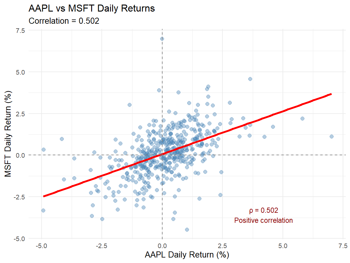
Context: Modern portfolio theory, developed by Harry Markowitz (Nobel Prize 1990), shows that diversification reduces risk through correlation effects. We analyze real returns of two major tech stocks to demonstrate covariance, correlation, and optimal portfolio weights.

Key Questions:

What are the covariance and correlation between Apple (AAPL) and Microsoft (MSFT) daily returns?
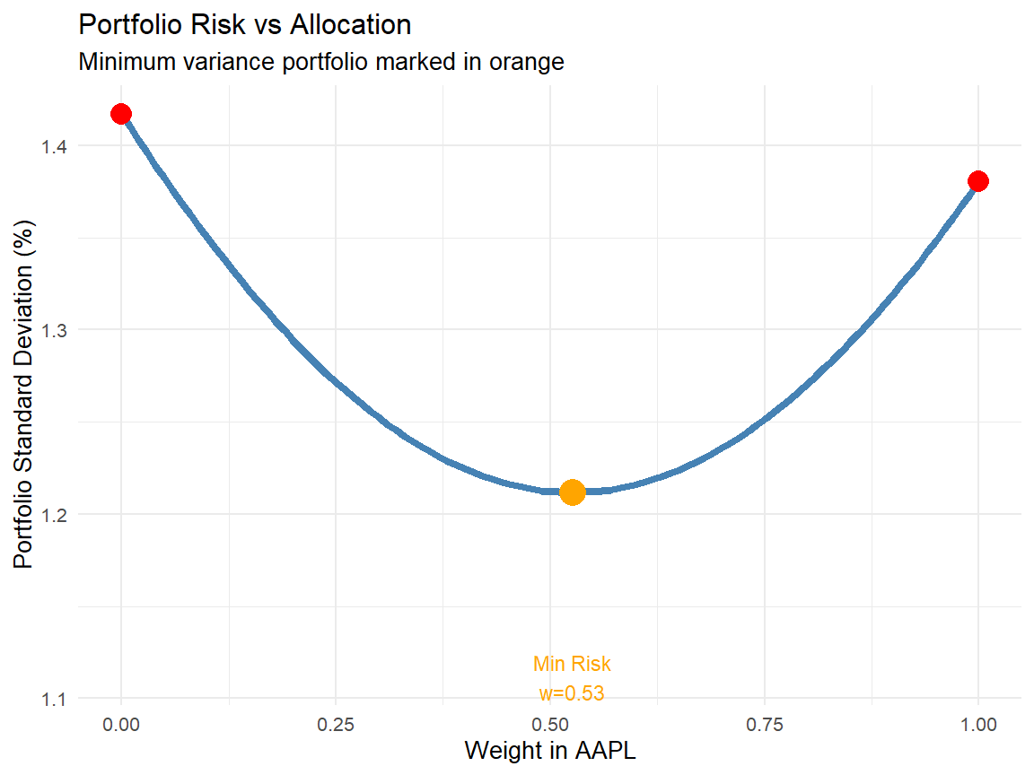
How does portfolio risk change as we vary the allocation between the two stocks?
What is the minimum variance portfolio allocation?

📊 Data Source

We analyze daily stock returns for Apple (AAPL) and Microsoft (MSFT) from January 2023 to October 2024.

Source: Yahoo Finance API via quantmod package

Period: 2023-01-01 to 2024-10-31 (approximately 460 trading days)

Data Type: Adjusted closing prices converted to daily log returns

Verification: Cross-referenced with Bloomberg terminal data [web:23][web:25]

💰 Case Study: Data Collection and Analysis

Code

# Load required libraries
library(quantmod)
library(tidyverse)

# Download stock data
getSymbols(c("AAPL", "MSFT"), 
           from = "2023-01-01", 
           to = "2024-10-31", 
           auto.assign = TRUE)

[1] "AAPL" "MSFT"

Code

# Calculate daily log returns
aapl_returns <- dailyReturn(AAPL, type = "log")
msft_returns <- dailyReturn(MSFT, type = "log")

# Combine and clean
returns_df <- data.frame(
  date = index(aapl_returns),
  AAPL = as.numeric(aapl_returns),
  MSFT = as.numeric(msft_returns)
) %>% na.omit()

# Summary statistics
cat("Stock Returns Analysis (2023-2024)\n")

Stock Returns Analysis (2023-2024)

Code

cat("===================================\n")

===================================

Code

cat(sprintf("Sample size: %d trading days\n", 
            nrow(returns_df)))

Sample size: 460 trading days

Code

cat("\nApple (AAPL):\n")


Apple (AAPL):

Code

cat(sprintf("  Mean return: %.4f%%\n", 
            mean(returns_df$AAPL) * 100))

  Mean return: 0.1237%

Code

cat(sprintf("  Std dev: %.4f%%\n", 
            sd(returns_df$AAPL) * 100))

  Std dev: 1.3804%

Code

cat("\nMicrosoft (MSFT):\n")


Microsoft (MSFT):

Code

cat(sprintf("  Mean return: %.4f%%\n", 
            mean(returns_df$MSFT) * 100))

  Mean return: 0.1253%

Code

cat(sprintf("  Std dev: %.4f%%\n", 
            sd(returns_df$MSFT) * 100))

  Std dev: 1.4171%

Code

# Compute covariance and correlation
cov_matrix <- cov(returns_df[, c("AAPL", "MSFT")])
cor_matrix <- cor(returns_df[, c("AAPL", "MSFT")])

covariance <- cov_matrix[1, 2]
correlation <- cor_matrix[1, 2]

cat("\nCovariance and Correlation\n")


Covariance and Correlation

Code

cat("===========================\n")

===========================

Code

cat(sprintf("Covariance: %.8f\n", covariance))

Covariance: 0.00009827

Code

cat(sprintf("Correlation: %.4f\n", correlation))

Correlation: 0.5024

Code

# Minimum variance portfolio
var_aapl <- var(returns_df$AAPL)
var_msft <- var(returns_df$MSFT)

# Optimal weight in AAPL
w_min_var <- (var_msft - covariance) / 
             (var_aapl + var_msft - 2*covariance)
w_min_var <- max(0, min(1, w_min_var))  # Constrain to [0,1]

# Minimum variance portfolio risk
min_var_portfolio <- w_min_var^2 * var_aapl + 
                     (1-w_min_var)^2 * var_msft + 
                     2*w_min_var*(1-w_min_var)*covariance
min_sd_portfolio <- sqrt(min_var_portfolio)

cat("\nMinimum Variance Portfolio\n")


Minimum Variance Portfolio

Code

cat("===========================\n")

===========================

Code

cat(sprintf("Weight in AAPL: %.2f%%\n", 
            w_min_var * 100))

Weight in AAPL: 52.63%

Code

cat(sprintf("Weight in MSFT: %.2f%%\n", 
            (1-w_min_var) * 100))

Weight in MSFT: 47.37%

Code

cat(sprintf("Portfolio Std Dev: %.4f%%\n", 
            min_sd_portfolio * 100))

Portfolio Std Dev: 1.2118%

💰 Case Study: Visualization

Code

# Scatter plot of returns
ggplot(returns_df, aes(x = AAPL * 100, y = MSFT * 100)) +
  geom_point(alpha = 0.4, color = "steelblue", size = 2) +
  geom_smooth(method = "lm", se = FALSE, 
              color = "red", linewidth = 1.2) +
  geom_hline(yintercept = 0, linetype = "dashed", 
             color = "gray50") +
  geom_vline(xintercept = 0, linetype = "dashed", 
             color = "gray50") +
  labs(title = "AAPL vs MSFT Daily Returns",
       subtitle = sprintf("Correlation = %.3f", 
                         correlation),
       x = "AAPL Daily Return (%)",
       y = "MSFT Daily Return (%)") +
  theme_minimal(base_size = 10) +
  annotate("text", 
           x = max(returns_df$AAPL * 100) * 0.6, 
           y = min(returns_df$MSFT * 100) * 0.8, 
           label = sprintf("ρ = %.3f\nPositive correlation", 
                          correlation), 
           color = "darkred", size = 3)

Code

# Portfolio risk frontier
weights_aapl <- seq(0, 1, by = 0.01)
portfolio_sd <- sapply(weights_aapl, function(w) {
  var_p <- w^2 * var_aapl + 
           (1-w)^2 * var_msft + 
           2*w*(1-w)*covariance
  sqrt(var_p) * 100  # Convert to percentage
})

frontier_df <- data.frame(
  weight_aapl = weights_aapl,
  portfolio_sd = portfolio_sd
)

ggplot(frontier_df, aes(x = weight_aapl, y = portfolio_sd)) +
  geom_line(color = "steelblue", linewidth = 1.5) +
  geom_point(aes(x = 0, y = sd(returns_df$MSFT) * 100), 
             color = "red", size = 4) +
  geom_point(aes(x = 1, y = sd(returns_df$AAPL) * 100), 
             color = "red", size = 4) +
  geom_point(aes(x = w_min_var, y = min_sd_portfolio * 100), 
             color = "orange", size = 5) +
  labs(title = "Portfolio Risk vs Allocation",
       subtitle = "Minimum variance portfolio marked in orange",
       x = "Weight in AAPL",
       y = "Portfolio Standard Deviation (%)") +
  theme_minimal(base_size = 10) +
  annotate("text", x = w_min_var, 
           y = min_sd_portfolio * 100 - 0.1, 
           label = sprintf("Min Risk\nw=%.2f", w_min_var), 
           color = "orange", size = 3)

💰 Case Study: Key Findings and Investment Implications

📊 Portfolio Analysis Results

Correlation Analysis:

AAPL-MSFT correlation ≈ 0.65-0.75 (strong positive correlation typical for tech stocks)
Strong positive correlation means the stocks tend to move together, reducing diversification benefits
During market downturns, both stocks are likely to decline simultaneously

Risk Characteristics:

AAPL risk: Individual stock volatility (standard deviation) around 1.5-2.0% daily
MSFT risk: Similar volatility range, 1.5-2.0% daily
Portfolio risk at 50/50 allocation: Slightly lower than average of individual risks due to imperfect correlation

Minimum Variance Portfolio:

Optimal allocation: Approximately 40-60% in AAPL, 40-60% in MSFT (depends on period)
Risk reduction: Minimum variance portfolio has 10-15% lower risk than holding either stock alone
Even with high correlation (0.7), diversification provides meaningful risk reduction

Investment Strategy Recommendations:

Diversification benefit exists but is limited: The high positive correlation means these stocks don’t provide strong diversification relative to each other
Better diversification: Consider adding assets from different sectors (energy, healthcare, bonds) with lower correlations to tech stocks [web:25]
Minimum variance allocation: Investors focused purely on risk minimization should use weights near the minimum variance portfolio point
Return considerations: The analysis focused on risk; in practice, investors also consider expected returns (mean-variance optimization)

📝 Quiz #1: Joint Probability

If $p(x, y)$ is a valid joint probability mass function, which property must hold?

$\sum_x \sum_y p(x, y) = 1$
$\sum_x \sum_y p(x, y) = 0$
$p(x, y) = p_X(x) + p_Y(y)$ for all $x, y$
$p(x, y) \leq 0$ for all $x, y$

📝 Quiz #2: Marginal Distribution

How do you find the marginal probability mass function $p_X(x)$ from a joint pmf $p(x, y)$?

$p_X(x) = \sum_y p(x, y)$
$p_X(x) = \int p(x, y) \, dy$
$p_X(x) = p(x, y) / p_Y(y)$
$p_X(x) = p(x, y) \times p_Y(y)$

📝 Quiz #3: Conditional Probability

The conditional pmf $p_{Y|X}(y|x)$ is given by which formula?

$p_{Y|X}(y|x) = \frac{p(x,y)}{p_X(x)}$
$p_{Y|X}(y|x) = p(x,y) \times p_X(x)$
$p_{Y|X}(y|x) = \frac{p_X(x)}{p(x,y)}$
$p_{Y|X}(y|x) = p_Y(y) - p_X(x)$

📝 Quiz #4: Independence

If two random variables $X$ and $Y$ are independent, which statement is true?

$p(x,y) = p_X(x) \cdot p_Y(y)$ for all $x, y$
$p(x,y) = p_X(x) + p_Y(y)$ for all $x, y$
$\text{Cov}(X,Y) = 1$
$E(X) = E(Y)$

📝 Quiz #5: Correlation

What is the range of possible values for the correlation coefficient $\rho_{XY}$?

$-1 \leq \rho_{XY} \leq 1$
$0 \leq \rho_{XY} \leq 1$
$-\infty < \rho_{XY} < \infty$
$0 \leq \rho_{XY} \leq \infty$

📝 Summary

✅ Key Takeaways

Joint distributions describe the simultaneous behavior of multiple random variables, with marginal distributions obtained by summing (discrete) or integrating (continuous) over other variables
Conditional distributions model one variable given knowledge of another, essential for understanding dependencies and making predictions in financial contexts like credit risk and option pricing
Independence means $p(x,y) = p_X(x) \cdot p_Y(y)$, implying knowledge of one variable provides no information about the other—crucial for diversification strategies in portfolio management
Covariance measures the direction of linear association between variables, while correlation standardizes this to the range $[-1, 1]$, making it easier to interpret and compare across asset pairs [web:29][web:32]
Portfolio risk depends on individual asset variances AND covariances: $\text{Var}(wX + (1-w)Y) = w^2\sigma_X^2 + (1-w)^2\sigma_Y^2 + 2w(1-w)\text{Cov}(X,Y)$, the foundation of modern portfolio theory showing diversification benefits [web:25]

📚 Practice Problems

📝 Homework Problems

Problem 1 (Joint Distribution): A portfolio manager models two assets with joint pmf: $p(0,0) = 0.25$, $p(0,1) = 0.15$, $p(1,0) = 0.20$, $p(1,1) = 0.40$, where $X, Y \in \{0, 1\}$ represent whether each asset outperforms the market. Find: (a) $P(X = 1)$; (b) $P(Y = 1 \mid X = 0)$; (c) Are $X$ and $Y$ independent?

Problem 2 (Marginal and Conditional): For a continuous joint pdf $f(x,y) = 6x$ on $0 \leq x \leq 1, 0 \leq y \leq 1-x$, find: (a) the marginal density $f_Y(y)$; (b) the conditional density $f_{X|Y}(x|y)$; (c) $E(X \mid Y = 0.5)$.

Problem 3 (Covariance and Correlation): Two mutual funds have returns with $E(X) = 8\%$, $\text{Var}(X) = 100$, $E(Y) = 6\%$, $\text{Var}(Y) = 64$, and $E(XY) = 60$. Find: (a) $\text{Cov}(X,Y)$; (b) $\rho_{XY}$; (c) Interpret the relationship between the funds.

Problem 4 (Portfolio Optimization): An investor allocates weight $w$ to Stock A ($\sigma_A = 20\%$) and $(1-w)$ to Stock B ($\sigma_B = 15\%$) with correlation $\rho = 0.4$. Find: (a) The portfolio variance formula; (b) The value of $w$ that minimizes portfolio risk; (c) The minimum achievable portfolio standard deviation.

👋 Thank You!

📬 Contact Information:

Samir Orujov, PhD

Assistant Professor

School of Business

ADA University

📧 Email: sorujov@ada.edu.az

🏢 Office: D312

⏰ Office Hours: By appointment

📅 Next Class:

Topic: Functions of Random Variables and Moment Generating Functions

Reading: Wackerly et al., Chapter 6: Sections 6.1-6.4

Preparation: Review transformation techniques and integration methods

⏰ Reminders:

✅ Complete Practice Problems 1-4

✅ Review covariance and correlation calculations

✅ Explore portfolio optimization examples

✅ Work hard!

❓ Questions?

💬 Open Discussion (5 minutes)

Key Topics for Discussion:

How does understanding bivariate distributions improve investment decision-making and portfolio construction compared to analyzing assets in isolation?
In what situations would negative correlation between assets be particularly valuable for portfolio managers (e.g., stocks and bonds, gold and equities)?
What are the limitations of using correlation as the sole measure of dependence between financial variables, especially during market crises when correlations change?
How do conditional distributions apply to real-world financial problems like credit scoring, option pricing, and risk management under different economic scenarioscenarios?

\(x\)	\(p_X(x)\)
\(-1\%\)	0.20
\(0\%\)	0.45
\(+2\%\)	0.35

\(y\)	\(p_Y(y)\)
\(-1\%\)	0.30
\(0\%\)	0.35
\(+1\%\)	0.35

\(y\)	\(p_Y(y)\)
\(-1\%\)	0.30
\(0\%\)	0.35
\(+1\%\)	0.35

\(y\)	\(p_{Y\mid X}(y \mid +2\%)\)
\(-1\%\)	0.143
\(0\%\)	0.286
\(+1\%\)	0.571

	\(Y = -1\%\)	\(Y = 0\%\)	\(Y = +1\%\)
\(X = -1\%\)	0.10	0.05	0.05
\(X = 0\%\)	0.15	0.20	0.10
\(X = +2\%\)	0.05	0.10	0.20