Mathematical Statistics

Expected Values, Covariance, and Correlation

Samir Orujov, PhD

ADA University, School of Business

Information Communication Technologies Agency, Statistics Unit

2026-02-22

🎯 Learning Objectives

By the end of this lecture, you will be able to:

• Compute expected values of functions of bivariate random variables using Definition 5.9

• Apply linearity properties (Theorems 5.6-5.8) to simplify expected value calculations

• Calculate covariance using both the definition and computational formula (Theorem 5.10)

• Compute and interpret the correlation coefficient as a standardized measure of linear association

• Apply the portfolio variance formula to analyze risk in multi-asset portfolios using real financial data

📱 Attendance Check-in

📋 Overview

📚 Topics Covered Today

• Expected Value of Functions – Definition 5.9 and computing \(E[g(Y_1, Y_2)]\)

• Theorems on Expected Values – Linearity and fundamental result \(E[Y_1 + Y_2] = E[Y_1] + E[Y_2]\)

• Covariance – Definition, interpretation, computational formula

• Correlation Coefficient – Standardized covariance and properties

• Case Study – Portfolio optimization with real data

📖 Motivation: Why Covariance and Correlation?

🎯 Measuring Relationships Between Variables

Understanding how two variables move together is fundamental in many applications:

Finance Applications:

• Do stock and bond returns move together or oppositely?
• How much does adding an asset reduce portfolio risk?
• What’s the systematic risk of an asset (beta)?

Other Applications:

• Does studying more hours improve exam scores?
• Are height and weight related?
• How does advertising spending relate to sales?

Key Question: How do we quantify the strength and direction of the linear relationship between two random variables?

📖 Definition: Expected Value of a Function

📝 Definition 5.9: Expected Value of \(g(Y_1, Y_2)\)

Let \(g(Y_1, Y_2)\) be a function of random variables \(Y_1\) and \(Y_2\).

Discrete Case: \[E[g(Y_1, Y_2)] = \sum_{y_1} \sum_{y_2} g(y_1, y_2) \cdot p(y_1, y_2)\]

Continuous Case: \[E[g(Y_1, Y_2)] = \int_{-\infty}^{\infty} \int_{-\infty}^{\infty} g(y_1, y_2) \cdot f(y_1, y_2) \, dy_1 \, dy_2\]

Key Insight: We can find the expected value of any function of \((Y_1, Y_2)\) by weighting function values by probabilities (discrete) or densities (continuous).

📌 Example 1: Computing \(E[Y_1 \cdot Y_2]\)

Problem: Let \(f(y_1, y_2) = 2y_1\) for \(0 < y_1 < 1\) and \(0 < y_2 < 1\). Find \(E[Y_1 \cdot Y_2]\).

Solution: Using Definition 5.9 with \(g(y_1, y_2) = y_1 \cdot y_2\):

\[E[Y_1 Y_2] = \int_0^1 \int_0^1 y_1 y_2 \cdot 2y_1 \, dy_1 \, dy_2\]

\[= \int_0^1 \int_0^1 2y_1^2 y_2 \, dy_1 \, dy_2 = \int_0^1 2y_2 \left[ \frac{y_1^3}{3} \right]_0^1 dy_2\]

\[= \int_0^1 \frac{2y_2}{3} \, dy_2 = \frac{2}{3} \left[ \frac{y_2^2}{2} \right]_0^1 = \frac{2}{3} \cdot \frac{1}{2} = \boxed{\frac{1}{3}}\]

Financial Context: If \(Y_1\) represents one asset’s return and \(Y_2\) another’s, \(E[Y_1 Y_2]\) is crucial for portfolio variance calculations.

📌 Example 2: Computing \(E[Y_1]\) from Joint Density

Problem: Using the same joint density \(f(y_1, y_2) = 2y_1\) on \([0,1] \times [0,1]\), find \(E[Y_1]\).

Method 1: Using marginal density

From Lecture 1: \(f_1(y_1) = \int_0^1 2y_1 \, dy_2 = 2y_1\)

\[E[Y_1] = \int_0^1 y_1 \cdot 2y_1 \, dy_1 = 2 \int_0^1 y_1^2 \, dy_1 = 2 \cdot \frac{1}{3} = \boxed{\frac{2}{3}}\]

Method 2: Using joint density directly

\[E[Y_1] = \int_0^1 \int_0^1 y_1 \cdot 2y_1 \, dy_2 \, dy_1 = \int_0^1 2y_1^2 \left[ y_2 \right]_0^1 dy_1 = \frac{2}{3}\]

Both methods give the same answer!

🧮 Theorems on Expected Values

Theorems 5.6-5.8: Linearity of Expected Value

Theorem 5.6: \(E[c] = c\) for any constant \(c\)

Theorem 5.7: \(E[c \cdot g(Y_1, Y_2)] = c \cdot E[g(Y_1, Y_2)]\)

Theorem 5.8: \(E[g_1(Y_1, Y_2) + g_2(Y_1, Y_2)] = E[g_1(Y_1, Y_2)] + E[g_2(Y_1, Y_2)]\)

🌟 Corollary: Fundamental Result

\[\boxed{E[Y_1 + Y_2] = E[Y_1] + E[Y_2]}\]

This holds always, regardless of whether \(Y_1\) and \(Y_2\) are independent!

More generally: \(E[aY_1 + bY_2 + c] = aE[Y_1] + bE[Y_2] + c\)

📌 Example 3: Expected Portfolio Return

Problem: An investor holds a portfolio with weight \(w_1 = 0.6\) in Stock A (expected return 8%) and \(w_2 = 0.4\) in Stock B (expected return 12%). Find the expected portfolio return.

Let \(Y_1\) = return on Stock A, \(Y_2\) = return on Stock B.

Portfolio return: \(R_p = w_1 Y_1 + w_2 Y_2 = 0.6 Y_1 + 0.4 Y_2\)

By linearity of expected value:

\[E[R_p] = E[0.6 Y_1 + 0.4 Y_2] = 0.6 E[Y_1] + 0.4 E[Y_2]\]

\[= 0.6(0.08) + 0.4(0.12) = 0.048 + 0.048 = \boxed{0.096 = 9.6\%}\]

Key Point: Expected portfolio return is simply the weighted average of individual expected returns—no covariance needed!

🧮 Theorem 5.9: Independence and Expected Values

Theorem 5.9: Product of Independent Variables

If \(Y_1\) and \(Y_2\) are independent, then for any functions \(g\) and \(h\):

\[E[g(Y_1) \cdot h(Y_2)] = E[g(Y_1)] \cdot E[h(Y_2)]\]

Special Case: \[E[Y_1 \cdot Y_2] = E[Y_1] \cdot E[Y_2] \quad \text{(if independent)}\]

Warning

Warning: The converse is NOT true! \(E[Y_1 Y_2] = E[Y_1] E[Y_2]\) does not imply independence.

Tip

Verification (Example 1): We found \(E[Y_1 Y_2] = 1/3\) and \(E[Y_1] = 2/3\).

For independent case: We’d also need \(E[Y_2] = 1/2\) (uniform on \([0,1]\)).

Check: \(E[Y_1] \cdot E[Y_2] = (2/3)(1/2) = 1/3 = E[Y_1 Y_2]\) ✓

📖 Definition: Covariance

📝 Definition 5.10: Covariance

The covariance of two random variables \(Y_1\) and \(Y_2\) is:

\[\text{Cov}(Y_1, Y_2) = E[(Y_1 - \mu_1)(Y_2 - \mu_2)]\]

where \(\mu_1 = E[Y_1]\) and \(\mu_2 = E[Y_2]\).

Interpretation:

• Positive covariance: Variables tend to deviate from their means in the same direction
• Negative covariance: Variables tend to deviate in opposite directions
• Zero covariance: No linear relationship (but variables may still be dependent!)

Notation: \(\text{Cov}(Y_1, Y_2) = \sigma_{12}\) or \(\sigma_{Y_1 Y_2}\)

🧮 Theorem 5.10: Computational Formula for Covariance

Theorem 5.10: Shortcut Formula

\[\text{Cov}(Y_1, Y_2) = E[Y_1 Y_2] - \mu_1 \mu_2 = E[Y_1 Y_2] - E[Y_1] \cdot E[Y_2]\]

Proof: \[\text{Cov}(Y_1, Y_2) = E[(Y_1 - \mu_1)(Y_2 - \mu_2)]\] \[= E[Y_1 Y_2 - \mu_2 Y_1 - \mu_1 Y_2 + \mu_1 \mu_2]\] \[= E[Y_1 Y_2] - \mu_2 E[Y_1] - \mu_1 E[Y_2] + \mu_1 \mu_2\] \[= E[Y_1 Y_2] - \mu_1 \mu_2 - \mu_1 \mu_2 + \mu_1 \mu_2 = E[Y_1 Y_2] - \mu_1 \mu_2\]

Key Insight: If \(Y_1\) and \(Y_2\) are independent, then \(E[Y_1 Y_2] = E[Y_1] E[Y_2]\), so \(\text{Cov}(Y_1, Y_2) = 0\).

📌 Example 4: Computing Covariance

Problem: For the joint density from Example 1, \(f(y_1, y_2) = 2y_1\) on \([0,1] \times [0,1]\), find \(\text{Cov}(Y_1, Y_2)\).

Solution:

From previous examples:

• \(E[Y_1] = 2/3\)
• \(E[Y_2] = 1/2\) (uniform on \([0,1]\))
• \(E[Y_1 Y_2] = 1/3\)

Using the computational formula:

\[\text{Cov}(Y_1, Y_2) = E[Y_1 Y_2] - E[Y_1] \cdot E[Y_2]\] \[= \frac{1}{3} - \frac{2}{3} \cdot \frac{1}{2} = \frac{1}{3} - \frac{1}{3} = \boxed{0}\]

Interpretation: Zero covariance confirms independence (from Theorem 5.5). Stock returns have no linear relationship.

📖 Definition: Correlation Coefficient

📝 Definition 5.11: Correlation Coefficient

The correlation coefficient between \(Y_1\) and \(Y_2\) is:

\[\rho = \rho_{Y_1, Y_2} = \frac{\text{Cov}(Y_1, Y_2)}{\sigma_1 \sigma_2}\]

where \(\sigma_1 = \sqrt{V(Y_1)}\) and \(\sigma_2 = \sqrt{V(Y_2)}\) are the standard deviations.

🌟 Properties of Correlation

1. Bounded: \(-1 \leq \rho \leq 1\) always
2. Dimensionless: No units, unlike covariance
3. Standardized: Same interpretation across different scales
4. Perfect linear relationship: \(|\rho| = 1\) if and only if \(Y_2 = a + bY_1\) for constants \(a, b\)

📌 Correlation Interpretation Guide

Correlation Values:

• \(\rho = +1\): Perfect positive linear
• \(\rho > 0.7\): Strong positive
• \(0.3 < \rho < 0.7\): Moderate positive
• \(-0.3 < \rho < 0.3\): Weak/no correlation
• \(\rho < -0.7\): Strong negative
• \(\rho = -1\): Perfect negative linear

Financial Examples:

• Stocks in same sector: \(\rho \approx 0.6-0.8\)
• Stocks and bonds: \(\rho \approx -0.2\) to \(+0.2\)
• Gold and USD: \(\rho \approx -0.3\) to \(-0.5\)
• S&P 500 vs individual stocks: \(\rho \approx 0.4-0.9\)

🧮 Theorem 5.11: Variance of Linear Combinations

Theorem 5.11: Portfolio Variance Formula

For any constants \(a\) and \(b\):

\[V(aY_1 + bY_2) = a^2 V(Y_1) + b^2 V(Y_2) + 2ab \text{ Cov}(Y_1, Y_2)\]

In terms of correlation:

\[V(aY_1 + bY_2) = a^2 \sigma_1^2 + b^2 \sigma_2^2 + 2ab\rho\sigma_1\sigma_2\]

Special Cases:

• If \(Y_1\) and \(Y_2\) are independent: \(\rho = 0\), so \(V(aY_1 + bY_2) = a^2 V(Y_1) + b^2 V(Y_2)\)
• For a portfolio with weights \(w_1\) and \(w_2\): \[\sigma_p^2 = w_1^2\sigma_1^2 + w_2^2\sigma_2^2 + 2w_1w_2\rho\sigma_1\sigma_2\]

📌 Example 5: Portfolio Standard Deviation

Problem: Portfolio with \(w_1 = 0.6\) in Stock A (\(\sigma_1 = 20\%\)) and \(w_2 = 0.4\) in Stock B (\(\sigma_2 = 15\%\)), with correlation \(\rho = 0.5\). Find portfolio standard deviation.

Solution: Using the portfolio variance formula:

\[\sigma_p^2 = w_1^2\sigma_1^2 + w_2^2\sigma_2^2 + 2w_1w_2\rho\sigma_1\sigma_2\]

\[= (0.6)^2(0.20)^2 + (0.4)^2(0.15)^2 + 2(0.6)(0.4)(0.5)(0.20)(0.15)\]

\[= 0.0144 + 0.0036 + 0.0072 = 0.0252\]

\[\sigma_p = \sqrt{0.0252} = 0.1587 = \boxed{15.87\%}\]

Key Insight: Portfolio risk (15.87%) < weighted average of individual risks (18%) due to diversification!

🤝 Think-Pair-Share Activity

💭 Diversification Paradox

Scenario: You have two investment options:

• Option A:

  • 100% in Stock X (\(\mu = 10\%\), \(\sigma = 25\%\))

• Option B:

  • 50% Stock X + 50% Stock Y (\(\mu_Y = 8\%\), \(\sigma_Y = 20\%\), \(\rho = -0.3\))

Questions:

1. Calculate expected return for both options
2. Calculate standard deviation for both options
3. Which option would you choose and why?

Activity: (3 minutes)

• 1 min: Think individually and calculate
• 1 min: Pair up and discuss your answers
• 1 min: Share key insights with class

🤝 Think-Pair-Share: Solutions

Expected Returns:

Option A:

\[E[R_A] = 10\%\]

Option B: \[E[R_B] = 0.5(10\%) + 0.5(8\%) = 9\%\]

Standard Deviations:

Option A:

\[\sigma_A = 25\%\]

Option B: \[\sigma_B^2 = (0.5)^2(0.25)^2 + (0.5)^2(0.20)^2\] \[+ 2(0.5)(0.5)(-0.3)(0.25)(0.20)\] \[= 0.015625 + 0.01 - 0.0075 = 0.018125\] \[\sigma_B = 13.46\%\]

Key Insight: Option B has lower return (9% vs 10%) but much lower risk (13.46% vs 25%)! The negative correlation provides powerful diversification. Most investors would prefer B for better risk-adjusted returns.

🎯 Minimum Variance Portfolio: The Optimization Problem

📝 Mathematical Formulation

Given:

• Two assets with standard deviations \(\sigma_1\) and \(\sigma_2\) (volatilities)
• Correlation coefficient \(\rho\) between the assets
• Portfolio weights: \(w_1\) and \(w_2\) where \(w_1 + w_2 = 1\)

Optimization Problem:

\[\min_{w_1, w_2} \quad \sigma_p^2 = w_1^2\sigma_1^2 + w_2^2\sigma_2^2 + 2w_1w_2\rho\sigma_1\sigma_2\]

\[\text{subject to:} \quad w_1 + w_2 = 1, \quad w_1, w_2 \geq 0 \text{ (no short selling)}\]

Solution (using calculus):

Substitute \(w_2 = 1 - w_1\), take derivative with respect to \(w_1\), and set to zero:

\[w_1^* = \frac{\sigma_2^2 - \rho\sigma_1\sigma_2}{\sigma_1^2 + \sigma_2^2 - 2\rho\sigma_1\sigma_2}, \quad w_2^* = 1 - w_1^*\]

Key Insight: Optimal weights depend on both variances and correlation!

📊 Interactive: Minimum Variance Portfolio vs Correlation

viewof rho_slider = {
  const input = Inputs.range([-1, 1], {
    value: 0.3,
    step: 0.1,
    label: "Correlation (ρ):",
    format: d => d.toFixed(2)
  });
  
  input.addEventListener('pointerdown', e => e.stopPropagation());
  input.addEventListener('touchstart', e => e.stopPropagation());
  input.addEventListener('mousedown', e => e.stopPropagation());
  input.addEventListener('click', e => e.stopPropagation());
  input.addEventListener('wheel', e => e.stopPropagation());
  input.addEventListener('pointermove', e => e.stopPropagation());
  input.addEventListener('touchmove', e => e.stopPropagation());
  
  return input;
}

sigma1 = 0.20  // 20% volatility for Asset 1
sigma2 = 0.15  // 15% volatility for Asset 2

// Calculate optimal minimum variance portfolio weight
// w1* = (σ₂² - ρσ₁σ₂) / (σ₁² + σ₂² - 2ρσ₁σ₂)
w1_optimal = (Math.pow(sigma2, 2) - rho_slider * sigma1 * sigma2) / 
             (Math.pow(sigma1, 2) + Math.pow(sigma2, 2) - 2 * rho_slider * sigma1 * sigma2)

// Constrain to [0, 1] (no short selling)
w1_star = Math.max(0, Math.min(1, w1_optimal))
w2_star = 1 - w1_star

// Minimum variance portfolio statistics
min_var = Math.pow(w1_star * sigma1, 2) + 
          Math.pow(w2_star * sigma2, 2) + 
          2 * w1_star * w2_star * rho_slider * sigma1 * sigma2

min_std = Math.sqrt(min_var)

// Generate efficient frontier data
weights = d3.range(0, 1.01, 0.01)
frontier_data = weights.map(w1 => {
  const w2 = 1 - w1;
  const var_p = Math.pow(w1 * sigma1, 2) + 
                Math.pow(w2 * sigma2, 2) + 
                2 * w1 * w2 * rho_slider * sigma1 * sigma2;
  return {
    w1: w1,
    std: Math.sqrt(var_p)
  };
})

Plot.plot({
  width: 820,
  height: 460,
  marginLeft: 60,
  marginBottom: 40,
  x: {
    label: "Weight in Asset 1",
    domain: [0, 1],
    grid: true
  },
  y: {
    label: "Portfolio Std Dev",
    tickFormat: d => `${(d * 100).toFixed(1)}%`,
    grid: true
  },
  marks: [
    Plot.line(frontier_data, {
      x: "w1", 
      y: "std", 
      stroke: "#2ecc71",
      strokeWidth: 3
    }),
    // Minimum variance portfolio point
    Plot.dot([{
      x: w1_star, 
      y: min_std
    }], {
      x: "x",
      y: "y",
      r: 8,
      fill: "#e74c3c",
      stroke: "#c0392b",
      strokeWidth: 2
    }),
    // Individual assets
    Plot.dot([
      {x: 0, y: sigma2, label: "Asset 2"},
      {x: 1, y: sigma1, label: "Asset 1"}
    ], {
      x: "x",
      y: "y",
      r: 5,
      fill: "#3498db"
    }),
    Plot.text([
      {x: 0.05, y: sigma2, label: "Asset 2", dx: 15},
      {x: 0.95, y: sigma1, label: "Asset 1", dx: 15}
    ], {
      x: "x",
      y: "y",
      text: "label",
      dx: "dx",
      fontSize: 12,
      fontWeight: "bold"
    }),
    // Label for minimum variance portfolio
    Plot.text([{
      x: w1_star, 
      y: min_std+0.005, 
      label: "Min Variance", 
      dy: -20
    }], {
      x: "x",
      y: "y",
      text: "label",
      dy: "dy",
      fontSize: 11,
      fontWeight: "bold",
      fill: "#e74c3c"
    })
  ]
})

html`<div style="text-align: center; font-size: 1.1em; margin-top: 10px;">
<strong>Minimum Variance Portfolio:</strong> w₁* = ${(w1_star * 100).toFixed(1)}%, 
w₂* = ${(w2_star * 100).toFixed(1)}% | 
σₚ = ${(min_std * 100).toFixed(2)}% | 
ρ = ${rho_slider.toFixed(2)}<br>
<em style="font-size: 0.9em;">Optimal weights change with correlation! Lower ρ → greater diversification benefit</em>
</div>`

💰 Case Study: Real Portfolio Data

Using real data from 2010-2024:

• SPY (S&P 500 ETF): Large-cap US stocks
• TLT (20+ Year Treasury Bond ETF): Long-term government bonds
• GLD (Gold ETF): Precious metals

library(tidyquant)
library(tidyverse)
library(knitr)

# Download monthly returns
symbols <- c("SPY", "TLT", "GLD")
prices <- tq_get(symbols, 
                 from = "2010-01-01", 
                 to = "2024-12-31",
                 get = "stock.prices")

# Calculate monthly returns
returns <- prices %>%
  group_by(symbol) %>%
  tq_transmute(select = adjusted,
               mutate_fun = periodReturn,
               period = "monthly",
               col_rename = "return")

# Convert to matrix format
returns_matrix <- returns %>%
  pivot_wider(names_from = symbol, values_from = return) %>%
  select(-date) %>%
  as.matrix()

# Compute statistics
cov_matrix <- cov(returns_matrix) * 12  # Annualize
cor_matrix <- cor(returns_matrix)

# Summary statistics
summary_stats <- data.frame(
  Asset = symbols,
  Mean = colMeans(returns_matrix) * 12 * 100,  # Annualized %
  StdDev = apply(returns_matrix, 2, sd) * sqrt(12) * 100,  # Annualized %
  Sharpe = (colMeans(returns_matrix) * 12) / (apply(returns_matrix, 2, sd) * sqrt(12))
)

kable(summary_stats, digits = 2, 
      caption = "Asset Statistics (2010-2024, Annualized)")

Asset Statistics (2010-2024, Annualized)

	Asset	Mean	StdDev	Sharpe
SPY	SPY	13.95	14.59	0.96
TLT	TLT	3.57	13.89	0.26
GLD	GLD	6.45	15.62	0.41

💰 Case Study: Correlation Matrix

# Display correlation matrix
kable(cor_matrix, digits = 3,
      caption = "Correlation Matrix")

Correlation Matrix

	SPY	TLT	GLD
SPY	1.000	-0.101	0.105
TLT	-0.101	1.000	0.262
GLD	0.105	0.262	1.000

📊 Key Observations

• SPY-TLT: Low/slightly negative correlation → good diversification
• SPY-GLD: Low positive correlation → some diversification benefit
• TLT-GLD: Moderate positive correlation → less diversification between these two

Investment Implication: Combining stocks (SPY) with bonds (TLT) provides excellent risk reduction due to low correlation.

💰 Case Study: Portfolio Analysis

# Define different portfolio allocations
portfolios <- list(
  "Equal Weight" = c(1/3, 1/3, 1/3),
  "60/40 (SPY/TLT)" = c(0.6, 0.4, 0.0),
  "Conservative" = c(0.3, 0.5, 0.2),
  "Aggressive" = c(0.7, 0.1, 0.2)
)

# Expected returns (annualized)
mu <- colMeans(returns_matrix) * 12

# Portfolio metrics
results <- data.frame(
  Portfolio = character(),
  ExpReturn = numeric(),
  StdDev = numeric(),
  Sharpe = numeric()
)

for(name in names(portfolios)) {
  w <- portfolios[[name]]
  port_return <- sum(w * mu)
  port_var <- t(w) %*% cov_matrix %*% w
  port_std <- sqrt(port_var)
  sharpe <- port_return / port_std
  
  results <- rbind(results, data.frame(
    Portfolio = name,
    ExpReturn = port_return * 100,
    StdDev = port_std * 100,
    Sharpe = sharpe
  ))
}

kable(results, digits = 2, row.names = FALSE)

Portfolio	ExpReturn	StdDev	Sharpe
Equal Weight	7.99	9.25	0.86
60/40 (SPY/TLT)	9.79	9.89	0.99
Conservative	7.26	9.24	0.79
Aggressive	11.41	11.05	1.03

library(ggplot2)

# Plot portfolios on risk-return space
ggplot(results, aes(x = StdDev, y = ExpReturn)) +
  geom_point(size = 4, color = "steelblue") +
  geom_text(aes(label = Portfolio), 
            vjust = -1, hjust = 0.5, size = 3) +
  geom_point(data = data.frame(
    StdDev = summary_stats$StdDev,
    ExpReturn = summary_stats$Mean
  ), color = "red", size = 3) +
  geom_text(data = data.frame(
    StdDev = summary_stats$StdDev,
    ExpReturn = summary_stats$Mean,
    label = c("SPY", "TLT", "GLD")
  ), aes(label = label), vjust = 1.5, 
  color = "red", size = 3) +
  labs(title = "Portfolio Risk-Return Analysis",
       subtitle = "Comparing allocation strategies",
       x = "Annualized Volatility (%)",
       y = "Expected Return (%)") +
  theme_minimal(base_size = 12) +
  xlim(0, max(summary_stats$StdDev) * 1.2)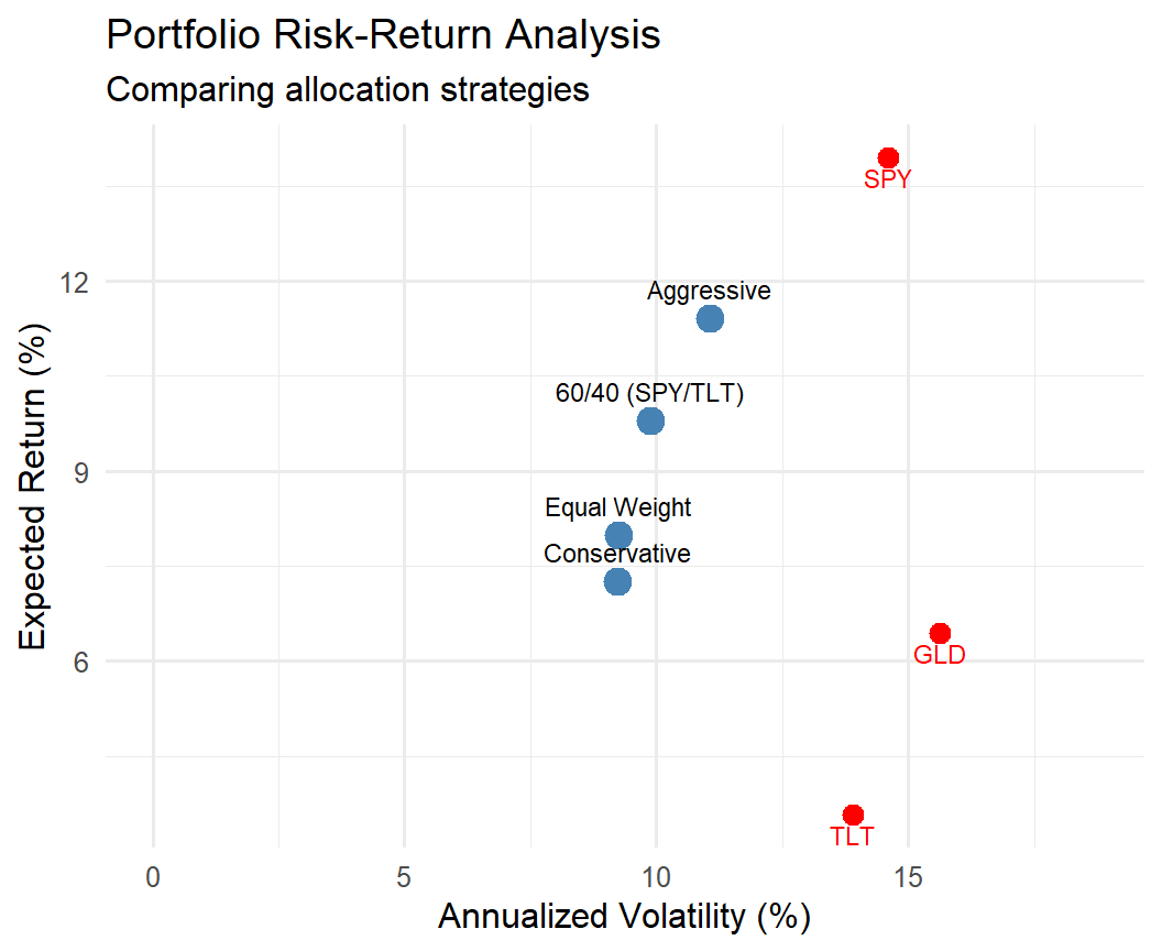

💰 Case Study: Key Findings

📊 Analysis Results

Correlation Insights:

• SPY-TLT: Low/negative → good diversification

• SPY-GLD: Low positive → some benefit

• TLT-GLD: Moderate positive

• Low correlations reduce risk

Portfolio Variance:

Equal-weight portfolio has lower risk:

\[\sigma_p^2 = \sum_i w_i^2 \sigma_i^2 \] \[+2\sum_{i<j} w_i w_j \rho_{ij} \sigma_i \sigma_j\]

Low/negative ρ reduces variance!

Investment Implications:

1. Diversification works

2. Correlation matters most

3. Trade-off: lower risk = lower return

📝 Quiz #1: Computing Expected Value

If \(E[Y_1] = 5\), \(E[Y_2] = 10\), what is \(E[3Y_1 + 2Y_2 - 7]\)?

• 28
• 35
• 22
• 15

📝 Quiz #2: Covariance Computation

If \(E[Y_1] = 2\), \(E[Y_2] = 3\), and \(E[Y_1 Y_2] = 7\), what is \(\text{Cov}(Y_1, Y_2)\)?

• 1
• 6
• 7
• -1

📝 Quiz #3: Independence and Covariance

Which statement about covariance is TRUE?

• If two variables are independent, their covariance must be zero
• If covariance is zero, the variables must be independent
• Covariance can be greater than 1
• Covariance equals correlation divided by the product of standard deviations

📝 Quiz #4: Portfolio Variance

For a portfolio with \(w_1 = w_2 = 0.5\), \(\sigma_1 = \sigma_2 = 20\%\), and \(\rho = 0\), what is the portfolio standard deviation?

• 14.14%
• 20%
• 10%
• 28.28%

📝 Summary

✅ Key Takeaways

• Expected value of functions \(E[g(Y_1, Y_2)]\) is computed by weighting function values by joint probabilities/densities

• Linearity: \(E[aY_1 + bY_2] = aE[Y_1] + bE[Y_2]\) always holds; \(E[Y_1 Y_2] = E[Y_1]E[Y_2]\) only if independent

• Covariance \(\text{Cov}(Y_1, Y_2) = E[Y_1 Y_2] - E[Y_1]E[Y_2]\) measures linear association

• Correlation \(\rho = \text{Cov}(Y_1, Y_2)/(\sigma_1 \sigma_2)\) is standardized with \(-1 \leq \rho \leq 1\)

• Critical insight: \(\text{Cov} = 0\) does NOT imply independence!

• Portfolio variance: \(V(w_1 Y_1 + w_2 Y_2) = w_1^2 V(Y_1) + w_2^2 V(Y_2) + 2w_1 w_2 \text{Cov}(Y_1, Y_2)\)

📚 Practice Problems

📝 Homework Problems

Problem 1: For \(f(y_1, y_2) = 8y_1y_2\) on \(0 < y_1 < 1\), \(0 < y_2 < 1\), find \(E[Y_1 + Y_2]\) and \(E[Y_1 Y_2]\).

Problem 2: For \(f(y_1, y_2) = 2\) on \(0 < y_1 < 1\), \(0 < y_2 < y_1\), compute \(\text{Cov}(Y_1, Y_2)\).

Problem 3: Two stocks: \(\sigma_1 = 30\%\), \(\sigma_2 = 20\%\), \(\text{Cov} = 0.024\). Find correlation.

Problem 4: Portfolio: \(w_1 = 0.4\), \(w_2 = 0.6\), \(\mu_1 = 12\%\), \(\mu_2 = 8\%\), \(\sigma_1 = 25\%\), \(\sigma_2 = 15\%\), \(\rho = 0.3\). Find expected return and standard deviation.

Problem 5: Verify for \(Y_1 \sim \text{Uniform}(-1, 1)\) and \(Y_2 = Y_1^2\): \(\text{Cov}(Y_1, Y_2) = 0\) but variables are dependent.

📱 Late Check-in

👋 Thank You!

📬 Contact Information:

Samir Orujov, PhD

Assistant Professor

School of Business

ADA University

📧 Email: sorujov@ada.edu.az

🏢 Office: D312

⏰ Office Hours: By appointment

📅 Next Class:

Topic: Functions of Random Variables (Chapter 6)

Reading: Chapter 6, Sections 6.1-6.3

Preparation: Review change of variables in calculus

⏰ Reminders:

✅ Complete Practice Problems 1-5

✅ Master the portfolio variance formula

✅ Remember: Cov = 0 ≠ independence!

✅ Work hard!

❓ Questions?

💬 Open Discussion

Key Topics for Discussion:

• Why is covariance so important in finance and portfolio theory?

• Can you think of examples where two variables have zero covariance but are clearly dependent?

• How would you estimate covariance from sample data? What are the challenges?

• What happens to diversification benefits during financial crises when correlations spike?