Mathematical Statistics

Multivariate Transformations and Order Statistics

Samir Orujov, PhD

ADA University, School of Business

Information Communication Technologies Agency, Statistics Unit

2026-02-22

🎯 Learning Objectives

By the end of this lecture, you will be able to:

Apply multivariate transformations using the Jacobian determinant to find joint distributions
Derive the distribution of sums and differences of random variables using Jacobians
Define and compute the distribution of order statistics \(Y_{(1)}, Y_{(2)}, \ldots, Y_{(n)}\)
Find the distribution of the sample range and other functions of order statistics
Apply order statistics to Value-at-Risk (VaR) and extreme value analysis in finance

📱 Attendance Check-in

📋 Overview

📚 Topics Covered Today

Multivariate Jacobian Transformations – Extending the change-of-variables technique to 2+ dimensions
The Jacobian Determinant – Computing \(|J|\) for bivariate transformations
Order Statistics – Distributions of sorted sample values
Extreme Order Statistics – \(Y_{(1)} = \min\) and \(Y_{(n)} = \max\)
Case Study – Value-at-Risk using order statistics

📖 Motivation: Multivariate Transformations

🎯 Why Study Multivariate Transformations?

Many important quantities involve functions of multiple random variables:

Statistical Applications:

Sum \(U = Y_1 + Y_2\) (sample total)
Ratio \(U = Y_1/Y_2\) (F-statistic)
Sample mean and variance jointly
Regression coefficients

Finance Applications:

Portfolio return = weighted sum
Sharpe ratio = return/volatility
Hedge ratio = covariance/variance
Option payoffs involving multiple assets

Key Question: Given joint distribution of \((Y_1, Y_2)\), find joint distribution of \((U_1, U_2) = (g_1(Y_1, Y_2), g_2(Y_1, Y_2))\).

📖 Definition: Bivariate Jacobian Transformation

📝 Theorem 6.6: Bivariate Transformation

Let \((Y_1, Y_2)\) have joint pdf \(f_{Y_1, Y_2}(y_1, y_2)\).

Define transformations: \(U_1 = g_1(Y_1, Y_2)\) and \(U_2 = g_2(Y_1, Y_2)\)

Let the inverse be: \(Y_1 = h_1(U_1, U_2)\) and \(Y_2 = h_2(U_1, U_2)\)

The Jacobian is: \[J = \begin{vmatrix} \frac{\partial y_1}{\partial u_1} & \frac{\partial y_1}{\partial u_2} \\ \frac{\partial y_2}{\partial u_1} & \frac{\partial y_2}{\partial u_2} \end{vmatrix} = \frac{\partial y_1}{\partial u_1}\frac{\partial y_2}{\partial u_2} - \frac{\partial y_1}{\partial u_2}\frac{\partial y_2}{\partial u_1}\]

Then: \[f_{U_1, U_2}(u_1, u_2) = f_{Y_1, Y_2}(h_1(u_1, u_2), h_2(u_1, u_2)) \cdot |J|\]

📌 Example 1: Sum and Difference

Problem: Let \(Y_1, Y_2\) be independent \(N(0, 1)\). Find the joint distribution of \(U_1 = Y_1 + Y_2\) and \(U_2 = Y_1 - Y_2\).

Solution:

Step 1: Find inverse transformation: \[y_1 = \frac{u_1 + u_2}{2}, \quad y_2 = \frac{u_1 - u_2}{2}\]

Step 2: Compute Jacobian: \[J = \begin{vmatrix} \frac{1}{2} & \frac{1}{2} \\ \frac{1}{2} & -\frac{1}{2} \end{vmatrix} = \frac{1}{2} \cdot \left(-\frac{1}{2}\right) - \frac{1}{2} \cdot \frac{1}{2} = -\frac{1}{2}\]

So \(|J| = \frac{1}{2}\)

Step 3: Apply formula. Since \(f_{Y_1,Y_2}(y_1, y_2) = \frac{1}{2\pi}e^{-(y_1^2 + y_2^2)/2}\):

\[f_{U_1,U_2}(u_1, u_2) = \frac{1}{2\pi}\exp\left[-\frac{(u_1+u_2)^2/4 + (u_1-u_2)^2/4}{2}\right] \cdot \frac{1}{2}\]

📌 Example 1: Sum and Difference (cont.)

Simplifying the exponent:

\[(u_1+u_2)^2 + (u_1-u_2)^2 = u_1^2 + 2u_1u_2 + u_2^2 + u_1^2 - 2u_1u_2 + u_2^2 = 2u_1^2 + 2u_2^2\]

So: \[f_{U_1,U_2}(u_1, u_2) = \frac{1}{4\pi}\exp\left[-\frac{u_1^2 + u_2^2}{4}\right]\]

\[= \frac{1}{2\sqrt{\pi}}e^{-u_1^2/4} \cdot \frac{1}{2\sqrt{\pi}}e^{-u_2^2/4}\]

Key Result

\(U_1 = Y_1 + Y_2 \sim N(0, 2)\) and \(U_2 = Y_1 - Y_2 \sim N(0, 2)\)

Moreover, \(U_1\) and \(U_2\) are independent!

📌 Example 2: Ratio of Normals

Problem: If \(Z_1, Z_2\) are independent \(N(0,1)\), find the distribution of \(T = Z_1/\sqrt{Z_2^2/1}\).

Solution outline:

This is related to the t-distribution. Set \(U_1 = Z_1\) and \(U_2 = Z_2^2\).

We know \(Z_2^2 \sim \chi^2(1)\), so: \[T = \frac{Z_1}{\sqrt{Z_2^2}} = \frac{N(0,1)}{\sqrt{\chi^2(1)/1}} \sim t(1)\]

Theorem 6.7: Student’s t-Distribution

If \(Z \sim N(0,1)\) and \(W \sim \chi^2(\nu)\) are independent, then: \[T = \frac{Z}{\sqrt{W/\nu}} \sim t(\nu)\]

The t-distribution with \(\nu\) degrees of freedom has pdf: \[f(t) = \frac{\Gamma((\nu+1)/2)}{\sqrt{\nu\pi}\Gamma(\nu/2)}\left(1 + \frac{t^2}{\nu}\right)^{-(\nu+1)/2}\]

📖 Definition: Order Statistics

📝 Definition 6.2: Order Statistics

Let \(Y_1, Y_2, \ldots, Y_n\) be a random sample from a distribution with pdf \(f(y)\) and CDF \(F(y)\).

The order statistics are the sample values arranged in ascending order: \[Y_{(1)} \leq Y_{(2)} \leq \cdots \leq Y_{(n)}\]

where: - \(Y_{(1)} = \min(Y_1, \ldots, Y_n)\) is the minimum - \(Y_{(n)} = \max(Y_1, \ldots, Y_n)\) is the maximum - \(Y_{(k)}\) is the \(k\)-th smallest value

Notation: Parentheses in subscript indicate ordered values!

🧮 Theorem: Distribution of Order Statistics

Theorem 6.8: PDF of the k-th Order Statistic

The pdf of \(Y_{(k)}\) is:

\[f_{Y_{(k)}}(y) = \frac{n!}{(k-1)!(n-k)!} [F(y)]^{k-1} [1-F(y)]^{n-k} f(y)\]

Intuition: - \([F(y)]^{k-1}\): probability that \(k-1\) observations are less than \(y\) - \([1-F(y)]^{n-k}\): probability that \(n-k\) observations are greater than \(y\) - \(f(y)\): one observation equals \(y\) - Multinomial coefficient: ways to arrange

Special Cases: - Minimum: \(f_{Y_{(1)}}(y) = n[1-F(y)]^{n-1}f(y)\) - Maximum: \(f_{Y_{(n)}}(y) = n[F(y)]^{n-1}f(y)\)

📌 Example 3: Maximum of Uniform Sample

Problem: Let \(Y_1, \ldots, Y_n\) be iid Uniform(0, 1). Find the distribution of \(Y_{(n)} = \max\).

Solution:

For Uniform(0,1): \(f(y) = 1\) and \(F(y) = y\) for \(0 < y < 1\).

Using the maximum formula: \[f_{Y_{(n)}}(y) = n[F(y)]^{n-1}f(y) = n \cdot y^{n-1} \cdot 1 = ny^{n-1}\]

for \(0 < y < 1\).

Properties:

\(E[Y_{(n)}] = \frac{n}{n+1}\)
As \(n \to \infty\), \(Y_{(n)} \to 1\)
This is Beta\((n, 1)\) distribution!

Financial Application:

Best return in a sample of \(n\) trading days — useful for performance attribution!

🎮 Interactive: Order Statistics Visualizer

Explore: Distribution of min and max from Uniform(0,1) samples

E[Y₍₁₎]:

E[Y₍ₙ₎]:

Range:

Code

orderPdfs = {
  const points = [];
  for (let y = 0.01; y <= 0.99; y += 0.01) {
    const f_min = n_order * Math.pow(1 - y, n_order - 1);
    const f_max = n_order * Math.pow(y, n_order - 1);
    points.push({y: y, f_min: f_min, f_max: f_max});
  }
  return points;
}

Plot.plot({
  width: 480,
  height: 320,
  x: { domain: [0, 1], label: "y" },
  y: { domain: [0, Math.max(n_order, 5)], label: "Density" },
  marks: [
    Plot.line(orderPdfs, {x: "y", y: "f_min", stroke: "red", strokeWidth: 2}),
    Plot.line(orderPdfs, {x: "y", y: "f_max", stroke: "blue", strokeWidth: 2}),
    Plot.ruleY([0])
  ]
})

Red: Minimum | Blue: Maximum

📖 Definition: Sample Range

📝 Definition 6.3: Sample Range

The sample range is defined as: \[R = Y_{(n)} - Y_{(1)} = \max - \min\]

Interpretation: Measures the spread of the sample data.

For a random sample from Uniform(0, \(\theta\)): - The range \(R\) is a sufficient statistic for \(\theta\) - \(E[R] = \frac{n-1}{n+1}\theta\)

Finance Application: The range of daily returns over a period measures realized volatility — the difference between the highest and lowest prices is the “trading range.”

🧮 Joint Distribution of Extreme Order Statistics

Theorem 6.9: Joint PDF of Min and Max

The joint pdf of \((Y_{(1)}, Y_{(n)})\) is:

\[f_{Y_{(1)}, Y_{(n)}}(y_1, y_n) = n(n-1)[F(y_n) - F(y_1)]^{n-2}f(y_1)f(y_n)\]

for \(y_1 < y_n\).

For Uniform(0,1): \[f_{Y_{(1)}, Y_{(n)}}(y_1, y_n) = n(n-1)(y_n - y_1)^{n-2}\]

This allows us to find the distribution of the range \(R = Y_{(n)} - Y_{(1)}\).

💰 Case Study: Value-at-Risk with Order Statistics

Code

library(tidyverse)
library(tidyquant)

# Download S&P 500 data
spy <- tq_get("SPY", from = "2015-01-01", to = "2024-12-31")

# Calculate daily returns
returns <- spy %>%
  mutate(ret = log(adjusted / lag(adjusted))) %>%
  na.omit()

n <- nrow(returns)
cat(sprintf("Sample size: %d trading days\n\n", n))

Sample size: 2514 trading days

Code

# Historical VaR using order statistics
# VaR at α = 5% means the α*n-th smallest return
alpha <- 0.05
k <- ceiling(alpha * n)  # k-th order statistic

sorted_returns <- sort(returns$ret)
var_5pct <- sorted_returns[k]

cat(sprintf("5%% Historical VaR: %.4f (%.2f%%)\n", 
            var_5pct, var_5pct * 100))

5% Historical VaR: -0.0169 (-1.69%)

Code

cat(sprintf("This is Y_(%d) from %d observations\n", k, n))

This is Y_(126) from 2514 observations

Code

# Also compute 1% VaR
k_1pct <- ceiling(0.01 * n)
var_1pct <- sorted_returns[k_1pct]
cat(sprintf("\n1%% Historical VaR: %.4f (%.2f%%)\n", 
            var_1pct, var_1pct * 100))


1% Historical VaR: -0.0325 (-3.25%)

Code

# Visualize VaR
ggplot(returns, aes(x = ret)) +
  geom_histogram(aes(y = after_stat(density)), 
                 bins = 100, fill = "steelblue", alpha = 0.7) +
  geom_vline(xintercept = var_5pct, color = "red", 
             linewidth = 1.2, linetype = "dashed") +
  geom_vline(xintercept = var_1pct, color = "darkred", 
             linewidth = 1.2, linetype = "dashed") +
  annotate("text", x = var_5pct - 0.005, y = 30, 
           label = "5% VaR", color = "red", angle = 90) +
  annotate("text", x = var_1pct - 0.005, y = 30, 
           label = "1% VaR", color = "darkred", angle = 90) +
  labs(title = "SPY Return Distribution with VaR",
       subtitle = "Historical VaR using order statistics",
       x = "Daily Log Return", y = "Density") +
  theme_minimal()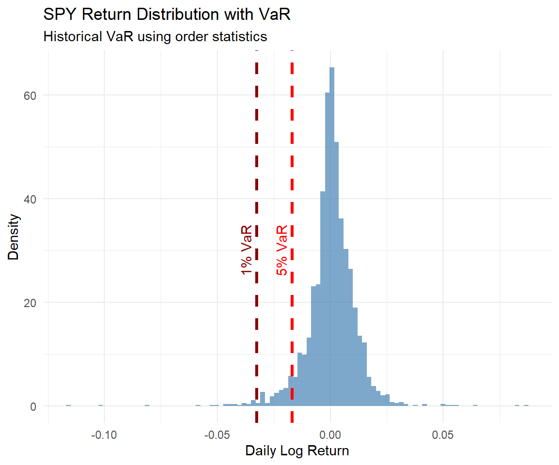

💰 Case Study: Extreme Returns Analysis

Code

# Analyze extreme returns (order statistics)
cat("=== Extreme Return Analysis ===\n\n")

=== Extreme Return Analysis ===

Code

# Worst 10 days (smallest order statistics)
cat("10 Worst Days (Y_(1) to Y_(10)):\n")

10 Worst Days (Y_(1) to Y_(10)):

Code

worst_10 <- returns %>%
  arrange(ret) %>%
  head(10) %>%
  select(date, ret)
print(worst_10, n = 10)

# A tibble: 10 × 2
   date           ret
   <date>       <dbl>
 1 2020-03-16 -0.116 
 2 2020-03-12 -0.101 
 3 2020-03-09 -0.0813
 4 2020-06-11 -0.0594
 5 2020-03-18 -0.0520
 6 2020-03-11 -0.0500
 7 2020-04-01 -0.0460
 8 2020-02-27 -0.0460
 9 2022-09-13 -0.0445
10 2020-03-20 -0.0440

Code

# Best 10 days (largest order statistics)  
cat("\n10 Best Days (Y_(n-9) to Y_(n)):\n")


10 Best Days (Y_(n-9) to Y_(n)):

Code

best_10 <- returns %>%
  arrange(desc(ret)) %>%
  head(10) %>%
  select(date, ret)
print(best_10, n = 10)

# A tibble: 10 × 2
   date          ret
   <date>      <dbl>
 1 2020-03-24 0.0867
 2 2020-03-13 0.0820
 3 2020-04-06 0.0650
 4 2020-03-26 0.0567
 5 2022-11-10 0.0535
 6 2020-03-17 0.0526
 7 2020-03-10 0.0505
 8 2018-12-26 0.0493
 9 2020-03-02 0.0424
10 2020-03-04 0.0412

Code

# Range statistics
range_ret <- max(returns$ret) - min(returns$ret)
cat(sprintf("\n=== Range Statistics ===\n"))


=== Range Statistics ===

Code

cat(sprintf("Maximum return: %.4f (%.2f%%)\n", 
            max(returns$ret), max(returns$ret)*100))

Maximum return: 0.0867 (8.67%)

Code

cat(sprintf("Minimum return: %.4f (%.2f%%)\n", 
            min(returns$ret), min(returns$ret)*100))

Minimum return: -0.1159 (-11.59%)

Code

cat(sprintf("Sample range: %.4f (%.2f%%)\n", 
            range_ret, range_ret*100))

Sample range: 0.2026 (20.26%)

Code

# Compare to theoretical for normal
sigma <- sd(returns$ret)
n <- nrow(returns)
# Expected range for normal is approximately 2*sigma*sqrt(2*log(n))
expected_range_normal <- 2 * sigma * sqrt(2 * log(n))
cat(sprintf("\nExpected range (if Normal): %.4f\n", expected_range_normal))


Expected range (if Normal): 0.0882

Code

cat(sprintf("Actual range: %.4f\n", range_ret))

Actual range: 0.2026

Code

cat(sprintf("Ratio: %.2f (>1 suggests fat tails)\n", 
            range_ret / expected_range_normal))

Ratio: 2.30 (>1 suggests fat tails)

💰 Case Study: Key Findings

📊 Analysis Results

Order Statistics for VaR:

5% VaR = \(Y_{(k)}\) where \(k = \lceil 0.05n \rceil\)
Non-parametric: no distribution assumption needed
Directly interpretable as “worst \(\alpha\)% of days”

Extreme Value Insights:

Worst days often cluster (market crises)
Best days also cluster (recovery periods)
Missing few best days dramatically hurts returns

Practical Implications:

Fat tails: Actual range exceeds normal prediction
Risk management: Order statistics provide robust VaR
Timing matters: Extreme days dominate long-term returns

📝 Quiz #1: Jacobian Transformation

For the transformation \(U_1 = Y_1 + Y_2\), \(U_2 = Y_1 - Y_2\), the absolute value of the Jacobian is:

📝 Quiz #2: Order Statistics Notation

In a sample of size \(n = 10\), \(Y_{(3)}\) represents:

The 3rd smallest value in the sample
The 3rd observation in the original sample
The 3rd largest value in the sample
The median of the sample

📝 Quiz #3: Maximum of Uniform Sample

If \(Y_1, \ldots, Y_5\) are iid Uniform(0,1), the pdf of \(Y_{(5)} = \max\) is:

\(5y^4\) for \(0 < y < 1\)
\(y^5\) for \(0 < y < 1\)
\(5(1-y)^4\) for \(0 < y < 1\)
\(1\) for \(0 < y < 1\)

📝 Quiz #4: Historical VaR

To compute the 5% historical VaR from 1000 daily returns, you would use:

The 50th smallest return (approximately \(Y_{(50)}\))
The 5th smallest return
The 950th smallest return
The average of all returns

📝 Summary

✅ Key Takeaways

Bivariate Jacobian: \(f_{U_1,U_2}(u_1,u_2) = f_{Y_1,Y_2}(h_1,h_2) \cdot |J|\) where \(J\) is the determinant of partial derivatives
Sum and difference of independent normals are independent normals — powerful result!
Order statistics \(Y_{(k)}\): k-th smallest value, with pdf involving \([F(y)]^{k-1}[1-F(y)]^{n-k}\)
Extreme order statistics: Min has pdf \(n[1-F(y)]^{n-1}f(y)\); Max has pdf \(n[F(y)]^{n-1}f(y)\)
Sample range \(R = Y_{(n)} - Y_{(1)}\) measures spread; useful for volatility estimation
Historical VaR: The \(\alpha\)-quantile is estimated by order statistic \(Y_{(\lceil \alpha n \rceil)}\)

📚 Practice Problems

📝 Homework Problems

Problem 1 (Jacobian): Let \(Y_1, Y_2\) be independent Exponential(1). Use Jacobian method to find the joint pdf of \(U = Y_1 + Y_2\) and \(V = Y_1/(Y_1 + Y_2)\). Show \(U\) and \(V\) are independent.

Problem 2 (Order Statistics): For a sample of size 5 from Exponential(β), find the pdf of the median \(Y_{(3)}\).

Problem 3 (Maximum): If \(Y_1, \ldots, Y_{10}\) are iid Exponential(1), find \(P(Y_{(10)} > 3)\).

Problem 4 (Range): For \(Y_1, \ldots, Y_n\) iid Uniform(0,1), find \(E[R]\) where \(R = Y_{(n)} - Y_{(1)}\).

Problem 5 (VaR): From 500 daily returns, you want to estimate the 1% VaR. Which order statistic would you use? What is the interpretation?

📱 Late Check-in

👋 Thank You!

📬 Contact Information:

Samir Orujov, PhD

Assistant Professor

School of Business

ADA University

📧 Email: sorujov@ada.edu.az

🏢 Office: D312

⏰ Office Hours: By appointment

📅 Next Class:

Topic: Sampling Distributions and the Central Limit Theorem (Chapter 7)

Reading: Chapter 7, Sections 7.1-7.3

Preparation: Review normal distribution properties

⏰ Reminders:

✅ Complete Practice Problems 1-5

✅ Review Chapter 6 concepts thoroughly

✅ Think about how sample statistics are distributed

✅ Work hard!

❓ Questions?

💬 Open Discussion

Key Topics for Discussion:

How does the Jacobian generalize the univariate transformation formula?
Why are order statistics useful for robust estimation?
What are the advantages of historical VaR over parametric VaR?
How do extreme value distributions extend order statistics theory?