Time Series Econometrics

Lecture 1: Stationarity, Ergodicity and White Noise

Samir Orujov, PhD

Open lecture notes, after Stanislav Anatolyev’s course (2016)

🎬 The Idea in 3 Minutes

A short film with the intuition. Watch it before the slides, or after. Captions: CC button.

🎯 Learning Objectives

By the end of this lecture, you will be able to:

• Explain why a time series is one trajectory of a process, and what that costs us
• Define strict stationarity and the strong, semi-strong and weak versions of white noise
• Derive the moments of MA(1), AR(1) and the random walk, and decide which are stationary
• Distinguish stationarity from ergodicity, with a process that has one but not the other
• Choose a transformation (log, difference, log return) that makes an economic series plausibly stationary

🗺️ Where We Are

This is the first lecture. The course asks one question over and over: what can we learn about a random process from a single stretch of its history?

• Lectures 1–3: the foundations — stationarity, ergodicity, the law of large numbers and the CLT for dependent data, and regression with time-series data
• Lectures 4–8: what to model, how to choose and evaluate models, and the linear (ARMA) workhorse
• Lectures 9–17: unit roots, nonlinear and regime models, VARs, volatility, breaks and risk

Today supplies the two assumptions everything else leans on.

❓ The Question

One history, one market

The S&P 500 has exactly one past. We cannot rerun 2016–2026 a thousand times to see how else it might have gone.

Yet we want to say “the expected daily return is about 0.05%” and attach a standard error to it. That means treating an average over time as if it were an average over possible histories.

When is that legitimate? The answer has two parts: stationarity and ergodicity.

👥 Two Kinds of Economist

	n-economist (cross-section)	t-economist (time series)
Data	\(\{x_i\}_{i=1}^{n}\)	\(\{x_t\}_{t=1}^{T}\)
What it is	\(n\) observations of one random variable	one segment of one realisation of \(\{x_t\}_{t=-\infty}^{+\infty}\)
Dependence	independent draws (i.i.d.)	not i.i.d.; we expect strong dependence
Asymptotics	\(n \to \infty\): more independent draws	\(T \to \infty\): a longer stretch of the same path

To apply large-sample theory to time series we must impose structure on the process \(\{x_t\}_{t=-\infty}^{+\infty}\). Without it, a single path says nothing about the space of paths it was drawn from.

🌌 The Space of Trajectories

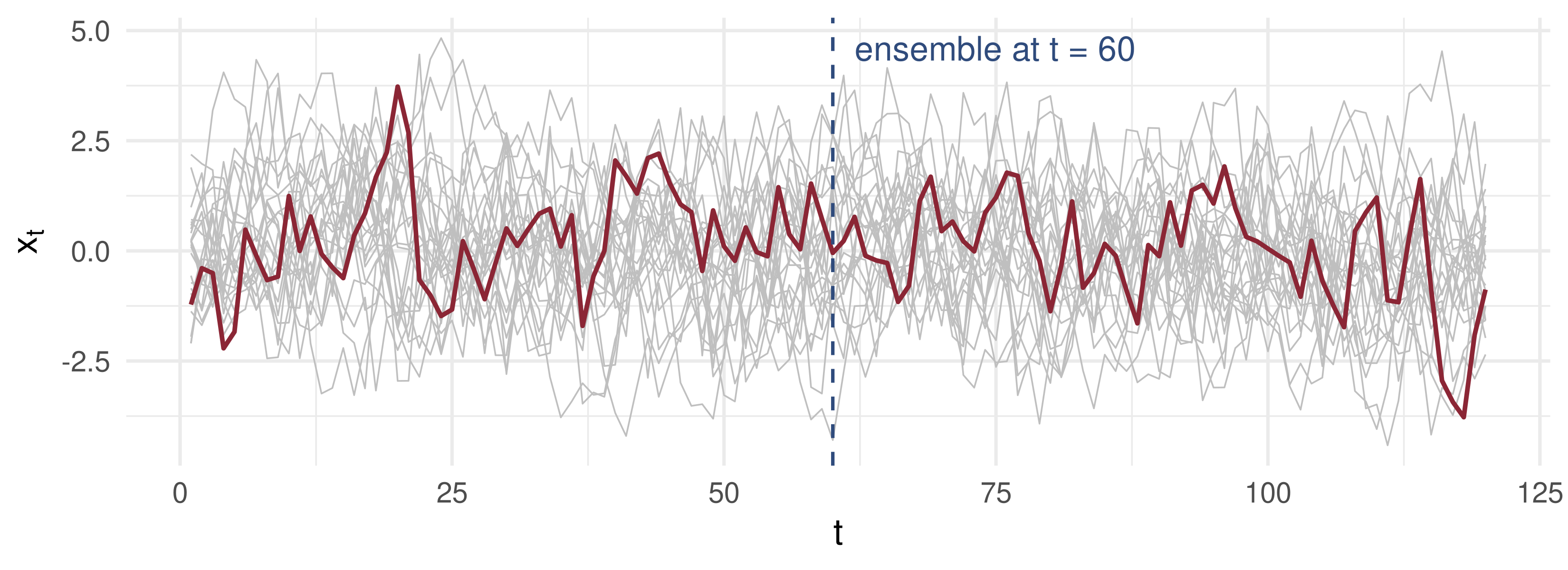
Grey: 25 possible histories. Red: the one we observe. \(E(x_t)\) is an average down the dashed line; the sample mean \(\bar x_T\) is an average along the red path.

📐 Strict Stationarity

Stationarity means that the statistical properties of the process are stable in time.

Definition (strict stationarity)

\(\{x_t\}\) is strictly stationary if, for every \(k \ge 0\), the joint distribution of \[(x_t,\ x_{t+1},\ \dots,\ x_{t+k})\] does not depend on \(t\).

So the distribution of \(x_t\) is the same for every \(t\); so is the joint distribution of every pair \((x_t, x_{t+j})\), every triple, and so on. In particular, if moments exist, \(E x_t = \mu\) and \(\operatorname{Cov}(x_t, x_{t+j}) = \Gamma_j\) depend on \(j\) only.

📐 White Noise: Three Strengths

Definitions

• Strong WN: \(\varepsilon_t \sim \text{iid}(0, \sigma^2)\) — the point where we are closest to the n-economist.
• Semi-strong WN: \(E(\varepsilon_t \mid \varepsilon_{t-1}, \varepsilon_{t-2}, \dots) = 0\) — the past does not help to predict \(\varepsilon_t\).
• Weak WN: \(E\varepsilon_t = 0\), \(\operatorname{Var}\varepsilon_t = \sigma^2\), \(\operatorname{Cov}(\varepsilon_t, \varepsilon_{t-k}) = 0\) for all \(k \ne 0\).

\[\text{strong} \;\Longrightarrow\; \text{semi-strong (if } \sigma^2<\infty) \;\Longrightarrow\; \text{weak}\]

Strong WN is strictly stationary. Weak WN need not be: only its first two moments are fixed in time. For instance, \(\varepsilon_t \sim N(0,1)\) for even \(t\) and \(\varepsilon_t \sim \pm 1\) with probability ½ each for odd \(t\) is weak WN, but its distribution changes from one period to the next.

📐 Why Semi-Strong Matters: Regression

The middle version is the one regression with time-series data needs: \[y_t = x_t'\beta + e_t, \qquad E\left(e_t \mid x_t, x_{t-1}, \dots,\ e_{t-1}, e_{t-2}, \dots\right) = 0.\]

• The error is unpredictable from current and past regressors and past errors.
• That is weaker than i.i.d. errors: the conditional variance of \(e_t\) may still move with the past.
• Lecture 3 shows that this condition is what makes OLS standard errors simple; when it fails, we need HAC standard errors.

🧮 Example: MA(1)

\(x_t = \varepsilon_t + \theta\varepsilon_{t-1}\), with \(\{\varepsilon_t\}\) white noise, variance \(\sigma^2\).

Mean. \(E x_t = E\varepsilon_t + \theta E\varepsilon_{t-1} = 0\).

Variance. The two shocks are uncorrelated, so \(\Gamma_0 = \operatorname{Var}x_t = (1 + \theta^2)\sigma^2\).

Lag 1. Only \(\varepsilon_t\) is shared by \(x_{t+1}\) and \(x_t\): \[\Gamma_1 = \operatorname{Cov}(\varepsilon_{t+1} + \theta\varepsilon_t,\ \varepsilon_t + \theta\varepsilon_{t-1}) = \theta\sigma^2.\]

Lag \(k \ge 2\). No shock in common, so \(\Gamma_k = 0\). None of these depends on \(t\): the MA(1) is stationary for every \(\theta\), and its memory ends after one period.

🧮 Example: AR(1) Is a Recursion

\(x_t = \rho x_{t-1} + \varepsilon_t\), \(\ |\rho| < 1\). Substitute the recursion into itself \(k\) times: \[x_t = \varepsilon_t + \rho\varepsilon_{t-1} + \dots + \rho^{k-1}\varepsilon_{t-k+1} + \rho^{k}x_{t-k}.\]

As \(k \to \infty\), \(\rho^k x_{t-k} \to 0\) for any path with bounded variance, which leaves the stationary solution \[x_t = \sum_{j=0}^{\infty}\rho^j\varepsilon_{t-j}, \qquad \Gamma_0 = \frac{\sigma^2}{1-\rho^2}, \qquad \Gamma_k = \rho^{|k|}\,\Gamma_0.\]

The recursion has other solutions. If \(x_t\) solves it, so does \(y_t = x_t + \rho^t\), since \(\rho^t = \rho\cdot\rho^{t-1}\). But \(E y_t = \rho^t\) changes with \(t\): \(y_t\) is not stationary. Only one solution is.

💻 Many Solutions, One Stationary

set.seed(2026)
rho <- 0.85; T_len <- 60; e <- rnorm(T_len)
solve_ar <- function(x0) { x <- numeric(T_len); prev <- x0
  for (t in 1:T_len) { x[t] <- rho * prev + e[t]; prev <- x[t] }; x }
df <- data.frame(t = rep(1:T_len, 3),
  x = c(solve_ar(10), solve_ar(0), solve_ar(-10)),
  start = rep(c("x0 = 10", "x0 = 0", "x0 = -10"), each = T_len))
ggplot(df, aes(t, x, colour = start)) + geom_line(linewidth = 1) +
  scale_colour_manual(values = c("#8b2635", "#2f4b7c", "#e09f3e"), name = NULL) +
  labs(x = "t", y = expression(x[t])) + theme(legend.position = "top")

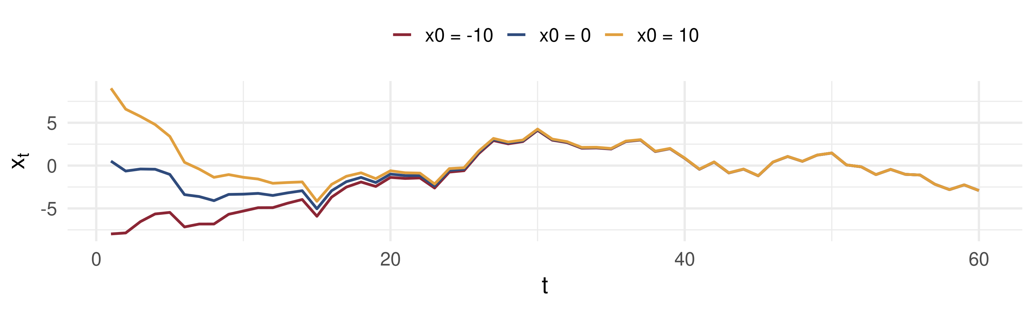
Same shocks, three starting values. The gaps are \(\pm 10\rho^t\): they die out, and every solution merges into the stationary one.

🧮 Example: The Random Walk

Set \(\rho = 1\): \(\ x_t = x_{t-1} + \varepsilon_t\), started at \(x_0 = 0\). Then \(x_t = \varepsilon_1 + \varepsilon_2 + \dots + \varepsilon_t\).

\[E x_t = 0, \qquad \operatorname{Var}(x_t) = t\sigma^2, \qquad \operatorname{Cov}(x_t, x_{t+k}) = t\sigma^2.\]

• The variance is not stable: it grows linearly with \(t\). The random walk is not stationary.
• The correlation \(\sqrt{t/(t+k)}\) between \(x_t\) and \(x_{t+k}\) tends to 1 as \(t\) grows: a shock is never forgotten. It is not ergodic either.
• Back-substitution fails for \(\rho = 1\): \(\rho^k x_{t-k} = x_{t-k}\) does not vanish, so there is no stationary solution to fall back on.

🌦️ What Breaks Stationarity?

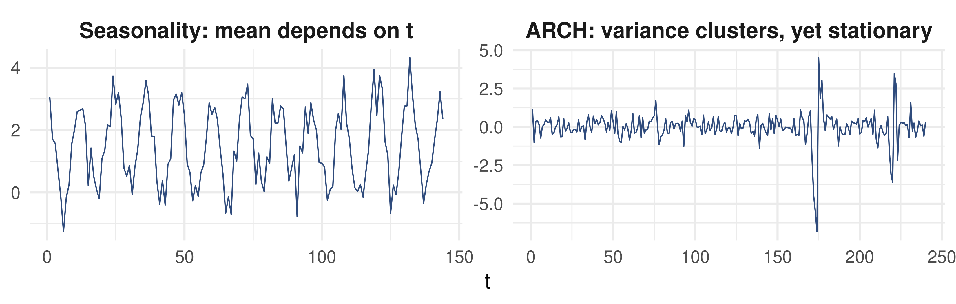
Left: monthly data whose winter and summer means differ, so the distribution of \(x_t\) depends on the season of \(t\) — not stationary. Right: \(\sigma_t^2 = 0.2 + 0.8\,\varepsilon_{t-1}^2\) moves with the past, but the unconditional variance \(0.2/(1-0.8) = 1\) is constant — stationary.

🎛️ Explore: Persistence

viewof rho = Inputs.range([-0.9, 1], {step: 0.01, value: 0.5, label: "AR coefficient ρ"})

ar_data = {
  const T = 500, rng = d3.randomNormal.source(d3.randomLcg(0.2026))(0, 1);
  const out = []; let x = 0, s = 0;
  for (let t = 1; t <= T; t++) {
    x = rho * x + rng(); s += x;
    out.push({t, value: x, series: "path x_t"});
    out.push({t, value: s / t, series: "running mean"});
  }
  return out;
}

Plot.plot({
  width: 1100, height: 300, marginLeft: 78, marginBottom: 50,
  style: {fontSize: "18px"},
  x: {label: "t"}, y: {label: null, grid: true},
  color: {domain: ["path x_t", "running mean"], range: ["#8ba3c7", "#8b2635"]},
  marks: [
    Plot.ruleY([0]),
    Plot.line(ar_data, {x: "t", y: "value", stroke: "series", strokeWidth: d => d.series === "running mean" ? 3 : 1.2})
  ]
})

Blue: the path \(x_t\); red: its running mean \(\bar x_t\). Same shocks for every \(\rho\). Near 0 the running mean settles at \(E x_t = 0\) quickly; near 1 it wanders for a long time; at \(\rho = 1\) it never settles.

📐 Ergodicity: Loss of Memory

Definition (heuristic)

\(\{x_t\}\) is ergodic if \(x_t\) and \(x_{t+k}\) become independent as \(k \to \infty\): the process loses its memory.

• Strictly, asymptotic independence is a mixing condition. It is sufficient for ergodicity, and it is the version to keep in mind.
• For asymptotic theory we require both stationarity and ergodicity (S&E).
• The random walk is neither stationary nor ergodic.
• Stationarity alone is not enough: the next slide has a stationary process with a perfect memory.

🧊 Stationary but Not Ergodic

Draw \(z \sim N(0,1)\) once, and set \(x_t = z\) for every \(t\).

• Stationary: every vector \((x_t, \dots, x_{t+k}) = (z, \dots, z)\) has the same distribution for every \(t\).
• Not ergodic: \(\operatorname{Cov}(x_t, x_{t-k}) = \operatorname{Var}(z) = 1\) for every \(k\). The dependence never dies out.

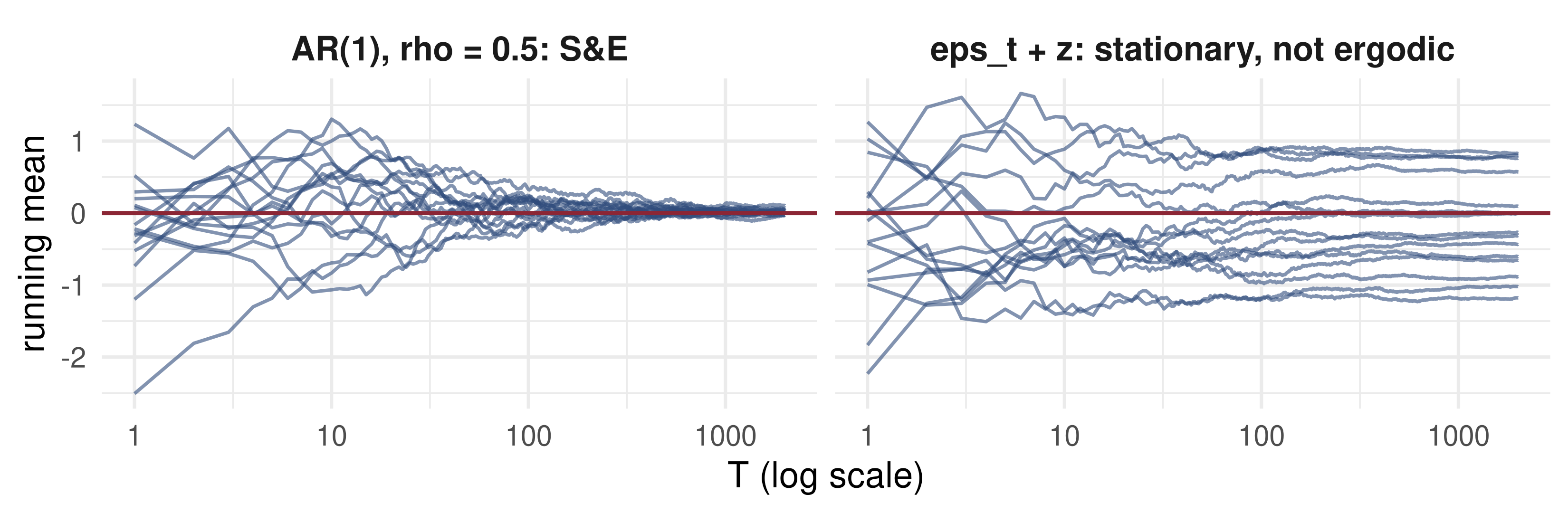
The sample mean is \(\bar x_T = z\) for every \(T\). It does not converge to \(E x_t = 0\). One path shows one value of \(z\), and no amount of waiting reveals the others.

A slightly richer version, \(x_t = \varepsilon_t + z\) with \(\varepsilon_t\) white noise, looks like noise on every path, yet each path hovers around its own level \(z\).

📐 The Law of Large Numbers

Law of large numbers for S&E series

If \(\{x_t\}\) is strictly stationary and ergodic and \(E|x_t| < \infty\), then \[\operatorname*{plim}_{T\to\infty}\ \frac1T\sum_{t=1}^{T}x_t = E(x_t).\]

This is the licence to replace an average over histories (the dashed line) by an average over time (the red path).

• For non-ergodic series the LLN does not hold.
• For non-stationary series \(E(x_t)\) is not even a single number to converge to.

💻 The LLN Working, and Failing

set.seed(2026)
T_len <- 2000; n_path <- 15; rho <- 0.5
run_mean <- function(x) cumsum(x) / seq_along(x)
erg <- replicate(n_path, run_mean(as.numeric(filter(rnorm(T_len), rho, "recursive"))))
non <- replicate(n_path, run_mean(rnorm(T_len) + rnorm(1)))   # x_t = eps_t + z
df <- rbind(
  data.frame(t = 1:T_len, m = as.vector(erg), p = rep(1:n_path, each = T_len), panel = "AR(1), rho = 0.5: S&E"),
  data.frame(t = 1:T_len, m = as.vector(non), p = rep(1:n_path, each = T_len), panel = "eps_t + z: stationary, not ergodic"))
ggplot(df, aes(t, m, group = p)) + geom_line(colour = "#2f4b7c", alpha = 0.6) +
  geom_hline(yintercept = 0, colour = "#8b2635", linewidth = 1) + facet_wrap(~ panel) +
  scale_x_log10() + labs(x = "T (log scale)", y = "running mean") +
  theme(strip.text = element_text(size = 17, face = "bold"))

Left: fifteen paths, one limit, \(E x_t = 0\). Right: fifteen paths, fifteen limits — each converges to its own \(z\), not to \(E x_t = 0\).

📐 Functions of S&E Series

Proposition

If \(\{x_t\}\) is S&E and \(f\) is a measurable function that does not depend on \(t\), then \[y_t = f(x_t, x_{t-1}, \dots, x_{t-n})\] is S&E. The same holds with infinitely many lags, provided the function is well defined.

• So \(x_t^2\), \(x_t x_{t-1}\), \(\log|x_t|\) and \(\mathbf 1\{x_t > 0\}\) inherit S&E from \(x_t\).
• MA(\(\infty\)). If \(\varepsilon_t\) is i.i.d. and \(\sum_j|\psi_j| < \infty\), then \(x_t = \sum_{j\ge0}\psi_j\varepsilon_{t-j}\) is S&E. With \(\psi_j = 0.9^j\) the sum converges: S&E.
• With \(\psi_j = 1\) for all \(j\) the sum does not converge, so \(f\) is not well defined; the partial sums form a random walk, neither S nor E.

🔧 Making a Series Stationary

Most economic levels are not stationary. We transform them first.

• Prices wander: use log returns \(r_t = \log P_t - \log P_{t-1}\).
• Output (GNP) grows exponentially, so its mean is growing. Take logs: \(\log \text{GNP}_t\) grows roughly linearly. Then difference: \[\Delta\log\text{GNP}_t = \log\frac{\text{GNP}_t}{\text{GNP}_{t-1}} \approx \frac{\Delta\text{GNP}_t}{\text{GNP}_{t-1}},\] the growth rate, which fluctuates around a constant mean.
• The trend in \(\log\text{GNP}\) may be deterministic or stochastic; telling them apart is the subject of Lectures 9–10.
• Seasonality and structural breaks also violate stationarity, and must be modelled rather than ignored.

🧠 Think–Pair–Share

\(\varepsilon_t\) is i.i.d. \(N(0,1)\); \(z \sim N(0,1)\) is drawn once, independent of \(\{\varepsilon_t\}\). For each process: is it strictly stationary? Is it ergodic?

1. \(x_t = \varepsilon_t + 3\varepsilon_{t-1}\)
2. \(x_t = z\,\varepsilon_t\)
3. \(x_t = \mu_{q(t)} + \varepsilon_t\), where \(q(t)\) is the quarter of month \(t\) and \(\mu_1, \dots, \mu_4\) are not all equal

Hint for 2: does \(\bar x_T\) converge to \(E x_t\)? Does the sample mean of \(x_t^2\)?

✅ Think–Pair–Share: Solution

1. S&E. An MA(1) is stationary for every \(\theta\), including \(\theta = 3\), and \(x_t\), \(x_{t+k}\) are independent once \(k \ge 2\).

2. Stationary, not ergodic. \((x_t, \dots, x_{t+k}) = z\,(\varepsilon_t, \dots, \varepsilon_{t+k})\), whose law does not depend on \(t\). The mean is fine: \(\bar x_T = z\,\bar\varepsilon_T \to 0 = E x_t\). But \[\frac1T\sum_t x_t^2 = z^2\,\frac1T\sum_t\varepsilon_t^2 \xrightarrow{p} z^2 \ne E x_t^2 = 1.\] \(|x_t|\) and \(|x_{t+k}|\) share \(|z|\) for every \(k\): the memory is in the scale.

3. Not stationary. \(E x_t = \mu_{q(t)}\) depends on \(t\). Removing the quarterly means (seasonal adjustment) gives back \(\varepsilon_t\), which is S&E.

💰 Case Study: Levels or Returns?

📈 The question

Is the S&P 500 a stationary series? If not, are its daily log returns?

1. Do the mean and standard deviation of the level stay put from one half of the sample to the other?
2. Do those of the returns?
3. What is left over that stationarity does not rule out?

📊 The data

Series: S&P 500 index, daily close (FRED SP500)

Period: 17 Oct 2016 – 14 Oct 2026, about 2,500 trading days

Transformation: \(r_t = 100\,(\log P_t - \log P_{t-1})\), in percent

# How the vendored file was obtained (not run here)
download.file("https://fred.stlouisfed.org/graph/fredgraph.csv?id=SP500", "data/SP500.csv")

💰 Case Study: Two Halves in R

sp <- read.csv("data/SP500.csv")
sp$P <- suppressWarnings(as.numeric(sp$SP500))   # FRED marks holidays "."
sp <- sp[!is.na(sp$P), ]
sp$date <- as.Date(sp$observation_date)
r <- 100 * diff(log(sp$P))                       # daily log returns, %
half <- rep(c("first half", "second half"), each = ceiling(length(r) / 2))[seq_along(r)]
lvl <- sp$P[-1]
acf1 <- function(x) acf(x, plot = FALSE)$acf[2]   # lag-1 autocorrelation
round(rbind(level_mean = tapply(lvl, half, mean), level_sd = tapply(lvl, half, sd),
            return_mean = tapply(r, half, mean),  return_sd = tapply(r, half, sd),
            acf1_return = tapply(r, half, acf1),  acf1_return_sq = tapply(r^2, half, acf1)), 3)

               first half second half
level_mean       3015.867    5345.921
level_sd          603.835    1188.593
return_mean         0.057       0.045
return_sd           1.210       1.069
acf1_return        -0.242      -0.016
acf1_return_sq      0.510       0.176

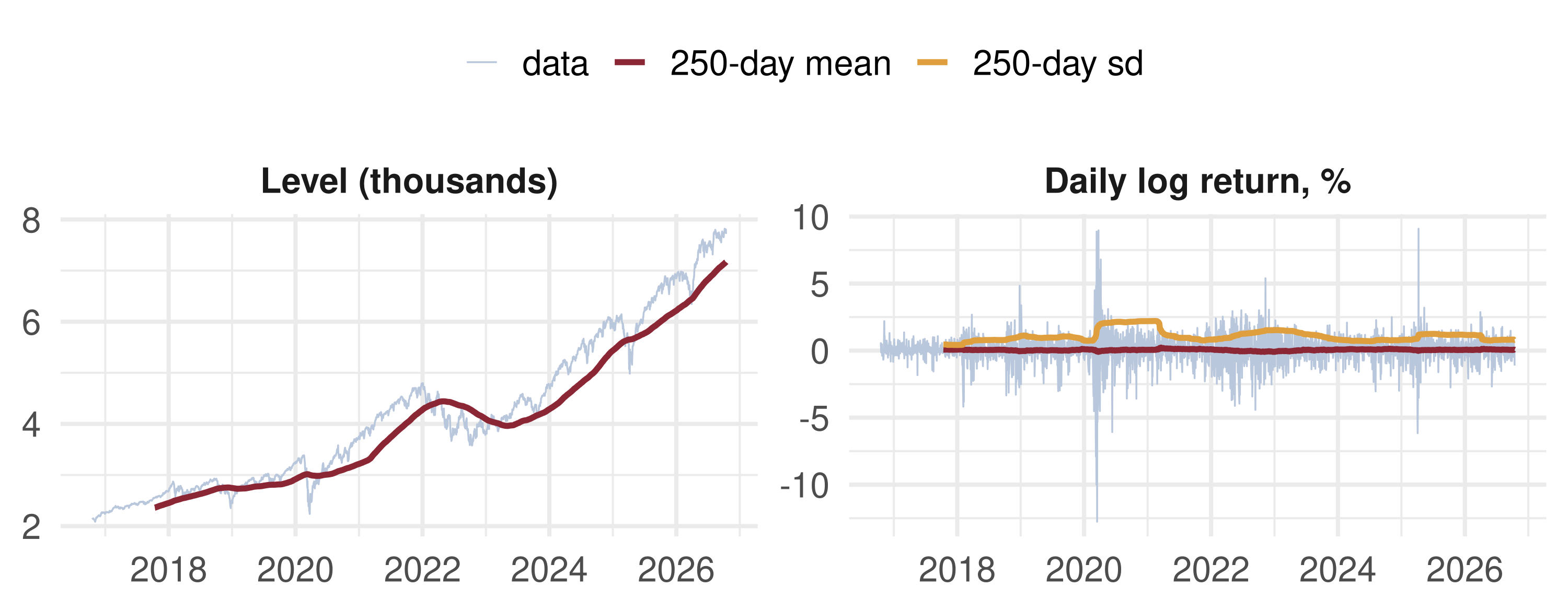
The level’s mean nearly doubles between halves; the return’s mean and sd barely move. Note the last row: \(r_t^2\) is clearly autocorrelated in both halves.

💰 Case Study: Rolling Windows

What the data say: the level trends upward, so its rolling mean has no fixed value to estimate; the returns fluctuate around a stable mean near zero, which is why we model returns. Stationarity is not the whole story: the rolling sd jumps in 2020 and stays high through 2022, and \(r_t^2\) is autocorrelated — volatility clustering, which a stationary but conditionally heteroskedastic model (Lecture 15) can capture.

📝 Quiz #1: Which White Noise?

\(\varepsilon_t = \sigma_t\eta_t\) with \(\eta_t\) i.i.d. \(N(0,1)\) and \(\sigma_t^2 = 0.2 + 0.5\,\varepsilon_{t-1}^2\). Which is the strongest version of white noise that \(\varepsilon_t\) satisfies?

• Strong: \(\varepsilon_t\) is i.i.d.
• Semi-strong: \(E(\varepsilon_t \mid \varepsilon_{t-1}, \dots) = 0\), but not i.i.d.
• Only weak: uncorrelated, but predictable in mean
• None: the variance changes over time

📝 Quiz #2: The Random Walk

\(x_t = x_{t-1} + \varepsilon_t\), \(x_0 = 0\), \(\operatorname{Var}\varepsilon_t = 4\). What is \(\operatorname{Var}(x_{25})\)?

• \(4\)
• \(\infty\)
• \(100\)
• \(4/(1-1^2)\), which is undefined

📝 Quiz #3: Stationary, Not Ergodic

\(x_t = \varepsilon_t + z\), with \(\varepsilon_t\) white noise and \(z \sim N(0,1)\) drawn once. As \(T \to \infty\), the sample mean \(\bar x_T\) converges in probability to …

• \(0 = E x_t\)
• \(z\), a random variable that differs from path to path
• Nothing: \(\bar x_T\) diverges
• \(1 = \operatorname{Var}(z)\)

📋 Key Formulas

Strict stationarity	law of \((x_t, \dots, x_{t+k})\) free of \(t\), every \(k\)
Strong / semi-strong / weak WN	iid\((0,\sigma^2)\) / \(E(\varepsilon_t\mid\text{past})=0\) / uncorrelated
MA(1)	\(\Gamma_0 = (1+\theta^2)\sigma^2\), \(\Gamma_1 = \theta\sigma^2\), \(\Gamma_k = 0\) for \(k\ge2\)
AR(1), \(\lvert\rho\rvert<1\)	\(x_t = \sum_{j\ge0}\rho^j\varepsilon_{t-j}\), \(\Gamma_k = \rho^{\lvert k\rvert}\sigma^2/(1-\rho^2)\)
Random walk, \(x_0 = 0\)	\(\operatorname{Var}x_t = t\sigma^2\)
LLN for S&E, \(E\lvert x_t\rvert<\infty\)	\(\frac1T\sum_{t=1}^T x_t \xrightarrow{p} E x_t\)
Log return / growth rate	\(\log P_t - \log P_{t-1} \approx \Delta P_t / P_{t-1}\)

📋 Summary

• A time series is one segment of one trajectory; to learn from it we impose stationarity and ergodicity
• Strict stationarity: every finite-dimensional distribution is invariant to shifts in time
• White noise comes in three strengths; the semi-strong (MDS) version is what time-series regression needs
• MA(1) is always stationary; AR(1) has a unique stationary solution when \(|\rho|<1\); the random walk has none
• Ergodicity is loss of memory; \(x_t = z\) is stationary with a perfect memory, and its sample mean never learns \(E x_t\)
• Under S&E the time average converges to the expectation; we transform levels (logs, differences, returns) to get there

📚 Further Reading

• Hamilton, J. D. (1994). Time Series Analysis. Princeton UP, ch. 3.1–3.2 (stationarity, ergodicity, white noise) and ch. 7.2 (the LLN for dependent data).
• Tsay, R. S. (2010). Analysis of Financial Time Series, 3rd ed. Wiley, ch. 1 and 2.1–2.4 (returns, stationarity, AR and MA basics).
• Franses, P. H. and van Dijk, D. (2000). Non-Linear Time Series Models in Empirical Finance. Cambridge UP, ch. 2 (stylised facts of returns).
• Hayashi, F. (2000). Econometrics. Princeton UP, §2.2 (ergodic stationarity, MDS).

Next lecture: Ergodic Theorem, CLT and the Long-Run Variance — how fast \(\bar x_T\) converges, and how to put a standard error on it when the data have memory.