Time Series Econometrics

Lecture 8: ARMA Models: Identification, Estimation, Forecasting

Samir Orujov, PhD

Open lecture notes, after Stanislav Anatolyev’s course (2016)

🎬 The Idea in 3 Minutes

⬅ Previous lecture: 7 · Linear Projection, Innovations and the Wold Decomposition

A short film with the intuition. Watch it before the slides, or after. Captions: CC button.

🎯 Learning Objectives

By the end of this lecture, you will be able to:

• Check stationarity and invertibility of an ARMA(\(p,q\)) from the roots of its lag polynomials
• Identify a tentative order from the sample ACF and PACF
• Estimate an AR by OLS or Yule–Walker and an ARMA by conditional least squares or Gaussian (Q)MLE
• Diagnose a fitted model with the Ljung–Box test
• Forecast \(h\) steps ahead and compute the forecast MSE and interval

This lecture is not in the 2016 notes. It is written from Hamilton (1994), ch. 3–5, and Tsay (2010), ch. 2, in the notation of lectures 7 and 9.

🔁 Warm-up from last time

\(x_t = \varepsilon_t + 4\varepsilon_{t-1}\) with \(\operatorname{var}\varepsilon_t = 1\). What is its Wold decomposition?

• \(x_t = \tilde\varepsilon_t + \tfrac14\tilde\varepsilon_{t-1}\) with \(\operatorname{var}\tilde\varepsilon_t = 16\)
• \(x_t = \varepsilon_t + 4\varepsilon_{t-1}\) itself, since \(\psi_0 = 1\)
• \(x_t = \tilde\varepsilon_t + \tfrac14\tilde\varepsilon_{t-1}\) with \(\operatorname{var}\tilde\varepsilon_t = 1/16\)
• It has none: the process is not stationary

🗺️ Where We Are

Lecture 7: every purely nondeterministic stationary series is an MA(\(\infty\)) in its least-squares innovations, \[x_t = \mu + \sum_{j\ge0}\psi_j\varepsilon_{t-j}.\]

From \(T\) observations we cannot estimate infinitely many \(\psi_j\). The ARMA model replaces the sequence \(\psi_j\) by a ratio of two short polynomials, \(\psi(L) = \theta(L)/\phi(L)\). Three questions follow, and they are the whole lecture: which orders \((p, q)\)? how to estimate the coefficients? how to forecast with them?

Not in the 2016 notes: added from Hamilton (1994), ch. 3.

❓ The Question

Where will the yield curve be in a year?

The term spread, 10-year minus 3-month Treasury yield, is one of the best recession predictors in macroeconomics. In September 2026 it stood near 0.9 percentage points. What is the best forecast for September 2027, and how wide must an honest 95% interval be?

A forecast without an interval is half an answer. ARMA models give both, and they give them from the series’ own past alone.

Not in the 2016 notes: added from Tsay (2010), ch. 2.

📐 The ARMA(\(p,q\)) Model

Definition

\(x_t\) is ARMA(\(p,q\)) if \(\ \phi(L)(x_t - \mu) = \theta(L)\varepsilon_t\), where \[\phi(L) = 1 - \phi_1L - \dots - \phi_pL^p, \qquad \theta(L) = 1 + \theta_1L + \dots + \theta_qL^q,\] with \(\varepsilon_t\) white noise \((0, \sigma^2)\) and no common roots of \(\phi\) and \(\theta\).

• Stationary (causal) iff all roots of \(\phi(z) = 0\) lie outside the unit circle. Then \(\psi(L) = \theta(L)/\phi(L)\) and \(\sum|\psi_j| < \infty\)
• Invertible iff all roots of \(\theta(z) = 0\) lie outside the unit circle. Then \(\varepsilon_t\) is the LS innovation (lecture 7)
• AR(1): root \(1/\rho\), so \(|\rho| < 1\). MA(1): root \(-1/\theta\), so \(|\theta| < 1\)

Not in the 2016 notes: added from Hamilton (1994), ch. 3.

📐 Second Moments

model	\(\gamma_0\)	autocorrelation \(\rho_j\)
AR(1)	\(\sigma^2/(1 - \rho^2)\)	\(\rho^j\)
MA(1)	\((1 + \theta^2)\sigma^2\)	\(\rho_1 = \theta/(1 + \theta^2)\), \(\ \rho_j = 0\) for \(j \ge 2\)
AR(\(p\))	from Yule–Walker	\(\rho_j = \phi_1\rho_{j-1} + \dots + \phi_p\rho_{j-p}\), \(j \ge 1\)
ARMA(1,1)	\(\dfrac{1 + 2\phi\theta + \theta^2}{1 - \phi^2}\sigma^2\)	\(\rho_1 = \dfrac{(1 + \phi\theta)(\phi + \theta)}{1 + 2\phi\theta + \theta^2}\), \(\ \rho_j = \phi\rho_{j-1}\), \(j \ge 2\)

The AR part fixes how the ACF decays; the MA part fixes only the first \(q\) values.

Not in the 2016 notes: added from Hamilton (1994), ch. 3.

📐 The Partial Autocorrelation Function

Definition

The PACF at lag \(k\), \(\alpha_{kk}\), is the last coefficient of the linear projection \[\operatorname{Proj}(x_t \mid 1, x_{t-1}, \dots, x_{t-k}) = \alpha_{k0} + \alpha_{k1}x_{t-1} + \dots + \alpha_{kk}x_{t-k}.\]

It is the correlation of \(x_t\) and \(x_{t-k}\) net of the lags in between. For an AR(\(p\)) and \(k > p\), the projection is the model itself, so \(\alpha_{kk} = 0\).

	ACF	PACF
AR(\(p\))	decays	cuts off after \(p\)
MA(\(q\))	cuts off after \(q\)	decays
ARMA(\(p,q\))	decays after lag \(q\)	decays after lag \(p\)

Not in the 2016 notes: added from Hamilton (1994), ch. 4.

💻 What the Patterns Look Like

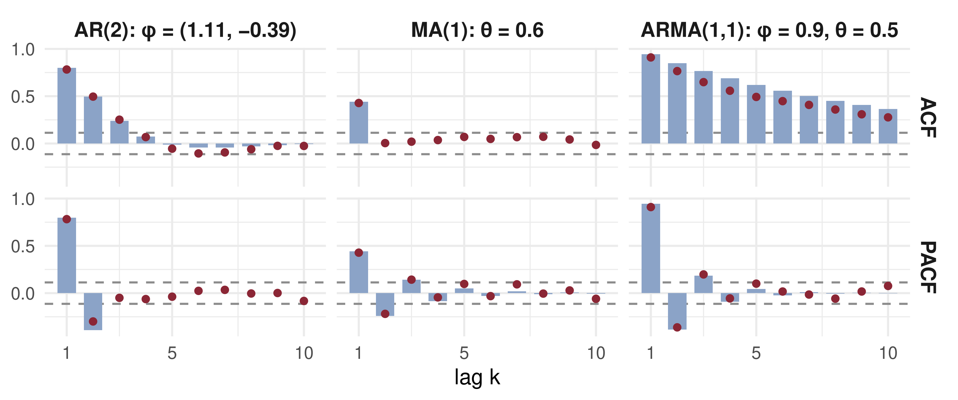
Bars: population values. Dots: one sample of \(T = 300\). Dashes: \(\pm1.96/\sqrt T\). Sampling noise blurs the cut-offs.

✏️ Yule–Walker for an AR(2)

Multiply \(x_t - \mu = \phi_1(x_{t-1} - \mu) + \phi_2(x_{t-2} - \mu) + \varepsilon_t\) by \(x_{t-j} - \mu\), \(j = 1, 2\), take expectations and divide by \(\gamma_0\): \[\rho_1 = \phi_1 + \phi_2\rho_1, \qquad \rho_2 = \phi_1\rho_1 + \phi_2.\] Suppose the sample gives \(\hat\rho_1 = 0.8\) and \(\hat\rho_2 = 0.5\).

Solve the two linear equations: \[\hat\phi_1 = \frac{\rho_1(1 - \rho_2)}{1 - \rho_1^2} = \frac{0.8 \cdot 0.5}{0.36} = 1.111, \qquad \hat\phi_2 = \frac{\rho_2 - \rho_1^2}{1 - \rho_1^2} = \frac{0.5 - 0.64}{0.36} = -0.389.\]

Not in the 2016 notes: added from Hamilton (1994), ch. 3.

✏️ The AR(2) Fit: Roots and Weights

Stationary? The AR(2) triangle: \(\phi_1 + \phi_2 = 0.722 < 1\), \(\ \phi_2 - \phi_1 = -1.5 < 1\), \(\ |\phi_2| < 1\). Yes.

Shape. \(\phi_1^2 + 4\phi_2 = -0.321 < 0\), so the roots of \(\phi(z)\) are complex with \(|z| = 1/\sqrt{-\phi_2} = 1.604 > 1\): a damped cycle.

Wold weights from \(\psi_j = \phi_1\psi_{j-1} + \phi_2\psi_{j-2}\): \(\ \psi_1 = 1.111\), \(\psi_2 = 0.846\), \(\psi_3 = 0.508\).

Innovation variance: \(\sigma^2 = \gamma_0(1 - \phi_1\rho_1 - \phi_2\rho_2) = 0.306\,\gamma_0\).

Not in the 2016 notes: added from Hamilton (1994), ch. 3.

💻 Checking the Example in R

r1 <- 0.8; r2 <- 0.5
phi <- solve(matrix(c(1, r1, r1, 1), 2), c(r1, r2))     # Yule-Walker system
roots <- polyroot(c(1, -phi))                            # roots of phi(z) = 1 - phi1 z - phi2 z^2
round(c(phi = phi, root_modulus = Mod(roots[1]),
        cycle_length = 2 * pi / abs(Arg(roots[1])),
        psi = ARMAtoMA(ar = phi, lag.max = 4),
        sigma2_over_gamma0 = 1 - sum(phi * c(r1, r2))), 3)

              phi1               phi2       root_modulus       cycle_length 
             1.111             -0.389              1.604             13.325 
              psi1               psi2               psi3               psi4 
             1.111              0.846              0.508              0.235 
sigma2_over_gamma0 
             0.306 

Roots of modulus 1.6 and a cycle of about 13 periods: a shock first overshoots, then oscillates back to the mean.

📐 Estimating an AR

• OLS of \(x_t\) on \(1, x_{t-1}, \dots, x_{t-p}\), conditioning on the first \(p\) observations. It is the sample analogue of the projection of lecture 7, so it is consistent under ergodicity, and asymptotically normal: for AR(1), \[\sqrt T(\hat\rho - \rho) \xrightarrow{d} N(0,\ 1 - \rho^2).\]
• Yule–Walker solves \(\rho_j = \sum_i\phi_i\rho_{j-i}\) with sample autocorrelations. Same limit as OLS, and the fit is always stationary
• With Gaussian errors, OLS is the conditional MLE

Not in the 2016 notes: added from Hamilton (1994), ch. 5, and Tsay (2010), ch. 2.

📐 Estimating MA and ARMA

The regressors \(\varepsilon_{t-j}\) are not observed, so OLS is out. Conditional sum of squares: set \(\varepsilon_0 = \dots = 0\), build residuals recursively, \[\varepsilon_t(\beta) = (x_t - \mu) - \sum_{i=1}^p\phi_i(x_{t-i} - \mu) - \sum_{j=1}^q\theta_j\varepsilon_{t-j}(\beta),\] and minimise \(\sum_t\varepsilon_t(\beta)^2\) numerically. The start-up error dies out only if \(\theta(L)\) is invertible: lecture 7’s picture again.

Gaussian MLE adds the density of the first observations (Kalman filter, Hamilton ch. 5). Under i.i.d. non-Gaussian errors it is a QMLE, still consistent and asymptotically normal.

Not in the 2016 notes: added from Hamilton (1994), ch. 5.

💻 Conditional Least Squares by Hand

x <- 1 + arima.sim(list(ar = 0.8, ma = 0.4), n = 500)   # ARMA(1,1), mu = 1
css <- function(b, x) {                                  # b = (mu, phi, theta)
  e <- numeric(length(x))
  for (t in 2:length(x)) e[t] <- (x[t] - b[1]) - b[2] * (x[t - 1] - b[1]) - b[3] * e[t - 1]
  sum(e[-1]^2)
}
fit <- optim(c(mean(x), 0, 0), css, x = x, method = "BFGS")
ref <- arima(x, order = c(1, 0, 1), method = "CSS")
rbind(truth = c(1, 0.8, 0.4), by_hand = fit$par,
      stats_arima = coef(ref)[c("intercept", "ar1", "ma1")]) |>
  `colnames<-`(c("mu", "phi", "theta")) |> round(3)

               mu   phi theta
truth       1.000 0.800 0.400
by_hand     0.715 0.785 0.441
stats_arima 0.715 0.785 0.441

A few lines of R reproduce the library’s estimator. The library’s method = "ML" adds the exact first-observation term.

Not in the 2016 notes: added from Hamilton (1994), ch. 5.

🔁 The Box–Jenkins Cycle

1. Identify. Transform to stationarity; read tentative \((p, q)\) from the ACF and PACF; shortlist with AIC/BIC (lecture 4)
2. Estimate by OLS, CSS or (Q)MLE
3. Check that residuals look like white noise. The Ljung–Box statistic \[Q(m) = T(T + 2)\sum_{k=1}^m\frac{\hat\rho_k^2(\hat\varepsilon)}{T - k} \xrightarrow{d} \chi^2(m - p - q)\] under correct specification. If it rejects, return to step 1
4. Forecast, and evaluate out of sample (lecture 5)

Parsimony is the rule: an ARMA(1,1) often does what an AR(5) does, with three parameters fewer.

Not in the 2016 notes: added from Box and Jenkins (1970) and Tsay (2010), ch. 2.

📐 Optimal Forecasts

Under squared loss the best forecast is the conditional mean; for a linear model with LS innovations it is the projection. From the Wold form, the future splits into known and unknown innovations: \[x_{T+h} = \mu + \underbrace{\sum_{j\ge h}\psi_j\varepsilon_{T+h-j}}_{\text{known at } T} + \underbrace{\sum_{j=0}^{h-1}\psi_j\varepsilon_{T+h-j}}_{\text{future}}\]

\[\hat x_{T+h|T} = \mu + \sum_{j\ge h}\psi_j\varepsilon_{T+h-j}, \qquad MSE(h) = \sigma^2\sum_{j=0}^{h-1}\psi_j^2 \ \xrightarrow[h\to\infty]{}\ \gamma_0.\] Forecasts revert to \(\mu\); the MSE rises to the unconditional variance. A 95% interval is \(\hat x_{T+h|T} \pm 1.96\sqrt{MSE(h)}\) under Gaussian errors, ignoring estimation error.

Not in the 2016 notes: added from Hamilton (1994), ch. 4.

✏️ AR(1) Forecast of the Spread

Monthly spread: \(\mu = 1.5\), \(\rho = 0.95\), \(\sigma = 0.3\), and an inverted curve today, \(x_T = -0.5\).

\[\hat x_{T+h|T} = \mu + \rho^h(x_T - \mu), \qquad MSE(h) = \sigma^2\,\frac{1 - \rho^{2h}}{1 - \rho^2}.\]

\(h\)	\(\hat x_{T+h\mid T}\)	\(\sqrt{MSE(h)}\)	95% interval
1	\(-0.40\)	\(0.30\)	\([-0.99,0.19]\)
6	\(0.03\)	\(0.65\)	\([-1.25,1.31]\)
12	\(0.42\)	\(0.81\)	\([-1.16,2.00]\)
\(\infty\)	\(1.50\)	\(0.96\)	\([-0.38,3.38]\)

After a year less than half the gap to \(\mu\) is closed; the interval is at 84% of its final width.

Not in the 2016 notes: added from Hamilton (1994), ch. 4.

💻 A Fan Converging to the Mean

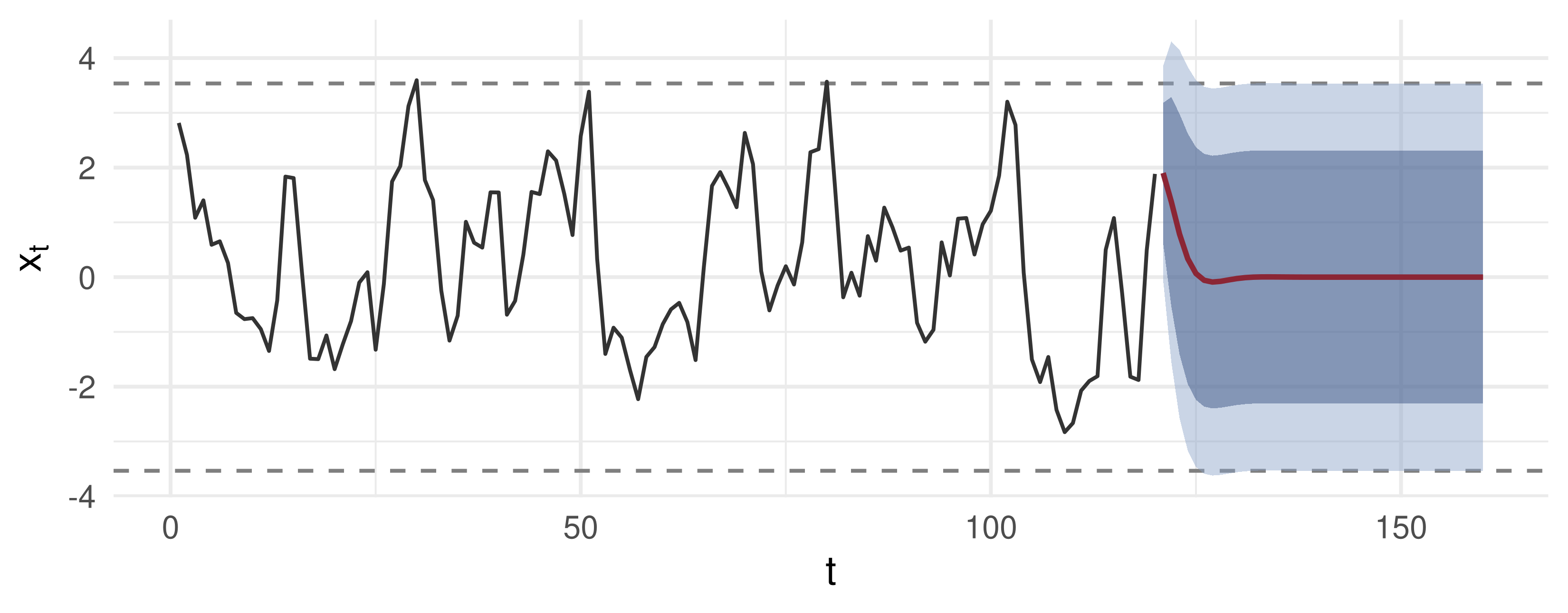
The AR(2) of the worked example. The point forecast (red) oscillates back to \(\mu\); the 80% and 95% bands widen to the unconditional band (dashes), \(\mu \pm 1.96\sqrt{\gamma_0}\).

🎛️ Explore: Persistence and the Fan

viewof rhoF = Inputs.range([0, 0.99], {step: 0.01, value: 0.95, label: "ρ"})

fanData = {
  const mu = 1.5, s = 0.3, xT = -0.5, out = [];
  for (let h = 0; h <= 36; h++) {
    const m = mu + Math.pow(rhoF, h) * (xT - mu);
    const se = h === 0 ? 0 : s * Math.sqrt((1 - Math.pow(rhoF, 2 * h)) / (1 - rhoF * rhoF));
    out.push({h, m, lo: m - 1.96 * se, hi: m + 1.96 * se});
  }
  return out;
}

Plot.plot({
  width: 1100, height: 330, marginLeft: 70, marginBottom: 55, marginTop: 30,
  style: {fontSize: "18px"},
  x: {label: "months ahead, h"}, y: {label: "spread, pp", domain: [-2.5, 5.5]},
  marks: [
    Plot.areaY(fanData, {x: "h", y1: "lo", y2: "hi", fill: "#8ba3c7", fillOpacity: 0.5}),
    Plot.ruleY([1.5], {stroke: "#888", strokeDasharray: "6,4"}),
    Plot.ruleY([1.5 - 1.96 * 0.3 / Math.sqrt(1 - rhoF * rhoF), 1.5 + 1.96 * 0.3 / Math.sqrt(1 - rhoF * rhoF)],
               {stroke: "#aaa", strokeDasharray: "2,4"}),
    Plot.line(fanData, {x: "h", y: "m", stroke: "#8b2635", strokeWidth: 3})
  ]
})

AR(1) from \(x_T = -0.5\), \(\mu = 1.5\), \(\sigma = 0.3\). Small \(\rho\): the forecast snaps to the mean and the band is narrow at once. As \(\rho \to 1\) both the reversion and the widening slow down, and the long-run band explodes.

🧠 Think-Pair-Share

\(x_t = 2 + \varepsilon_t + 0.6\,\varepsilon_{t-1}\), \(\ \sigma^2 = 1\), and the last innovation was \(\hat\varepsilon_T = 0.5\).

1. Compute \(\hat x_{T+1|T}\), \(\hat x_{T+2|T}\) and their MSEs.
2. Why is the two-step forecast no better than the unconditional mean?
3. A series has PACF \(0.90, -0.40, 0.02, 0.01\) and a slowly decaying, oscillating ACF. Which model would you try first?

✅ Think-Pair-Share: Solution

1. \(\hat x_{T+1|T} = 2 + 0.6 \cdot 0.5 = 2.3\), \(\ MSE(1) = \sigma^2 = 1\). \(\ \hat x_{T+2|T} = 2\), \(\ MSE(2) = (1 + 0.6^2)\sigma^2 = 1.36\).

2. \(\psi_j = 0\) for \(j \ge 2\): nothing known at \(T\) affects \(x_{T+2}\). The MSE has already reached \(\gamma_0 = 1.36\). An MA(\(q\)) has memory of exactly \(q\) periods.

3. PACF cuts off after lag 2 and the ACF decays: an AR(2). The negative \(\alpha_{22}\) with an oscillating ACF points to complex roots, as in the worked example.

Not in the 2016 notes: added from Hamilton (1994), ch. 4.

💰 Case Study: The Term Spread

📈 The question

1. Which ARMA order do the ACF, PACF and BIC point to?
2. Are its residuals white noise (Ljung–Box)?
3. What is the 12-month forecast, and how wide is its 95% interval?

📊 The data

Series: 10-year minus 3-month Treasury yield, FRED T10Y3M

Period: Jan 1982 – Sep 2026, 537 months

Transformation: monthly average of daily values, percentage points

read.csv("https://fred.stlouisfed.org/
  graph/fredgraph.csv?id=T10Y3M")

💰 Case Study: Identify, Estimate, Check

d <- read.csv("data/T10Y3M.csv")
d$T10Y3M <- suppressWarnings(as.numeric(d$T10Y3M))       # FRED marks holidays with "."
d <- na.omit(d); d$month <- substr(d$observation_date, 1, 7)
m <- aggregate(T10Y3M ~ month, data = d, FUN = mean); x <- m$T10Y3M
cands <- list("AR(1)" = c(1, 0, 0), "AR(2)" = c(2, 0, 0), "AR(3)" = c(3, 0, 0),
              "ARMA(1,1)" = c(1, 0, 1), "ARMA(2,1)" = c(2, 0, 1))
fits <- lapply(cands, function(o) arima(x, order = o, method = "ML"))
tab  <- t(sapply(names(fits), function(k) c(BIC = BIC(fits[[k]]),
          LjungBox_p = Box.test(resid(fits[[k]]), lag = 24, type = "Ljung-Box",
                                fitdf = sum(cands[[k]]))$p.value)))
best <- fits[[which.min(tab[, "BIC"])]]; fc <- predict(best, n.ahead = 24)
f2 <- function(v) paste(sprintf("%5.2f", v), collapse = " ")
cat("ACF,  lags 1-4:", f2(acf(x, 4, plot = FALSE)$acf[2:5]),
    "\nPACF, lags 1-4:", f2(pacf(x, 4, plot = FALSE)$acf[1:4]), "\n\n",
    paste(capture.output(print(round(tab, 3))), collapse = "\n"),
    "\n\nbest:", names(fits)[which.min(tab[, "BIC"])], " coef:", f2(coef(best)),
    "\nh = 12: forecast", f2(fc$pred[12]), " 95% interval",
    f2(fc$pred[12] + c(-1.96, 1.96) * fc$se[12]), "\n")

ACF,  lags 1-4:  0.98  0.94  0.90  0.86 
PACF, lags 1-4:  0.98 -0.32  0.13 -0.06 

               BIC LjungBox_p
AR(1)     139.979      0.000
AR(2)      81.693      0.006
AR(3)      73.451      0.234
ARMA(1,1)  63.802      0.390
ARMA(2,1)  69.846      0.360 

best: ARMA(1,1)  coef:  0.96  0.45  1.53 
h = 12: forecast  1.18  95% interval -0.74  3.10 

💰 Case Study: The Forecast Fan

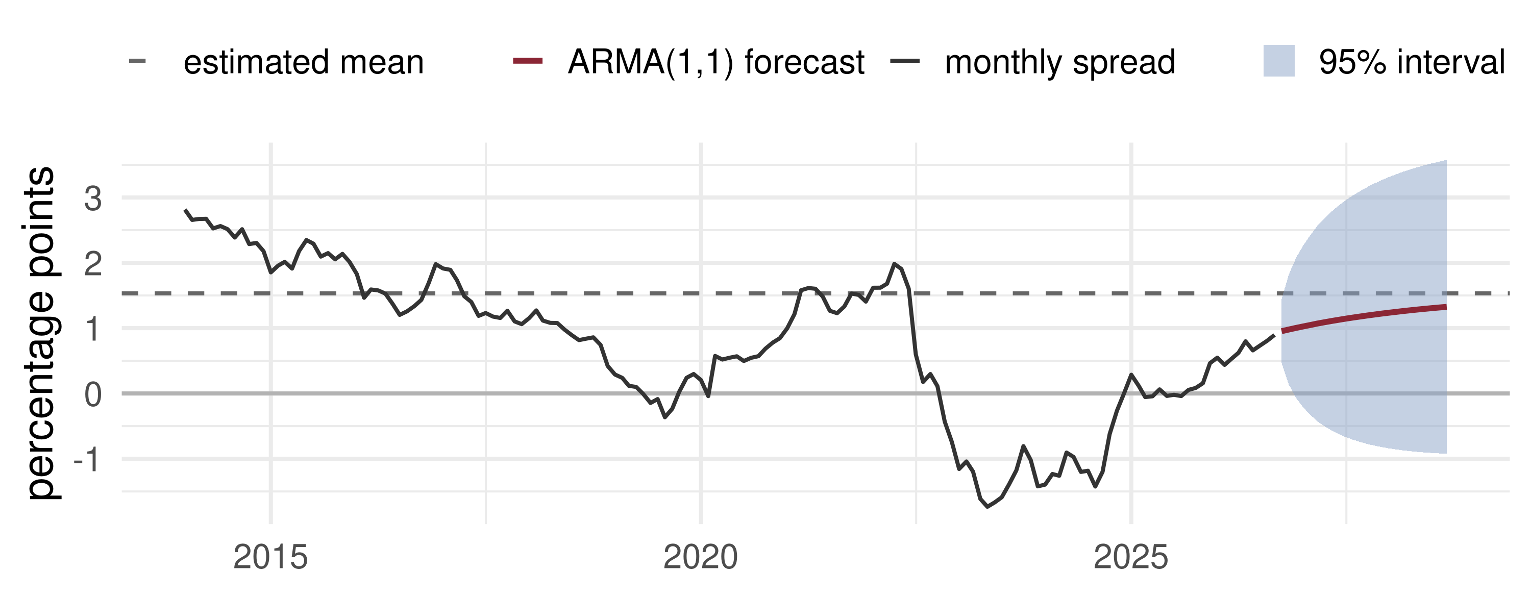
What the data say: the PACF suggests AR(2), but AR(2) fails Ljung–Box; ARMA(1,1) has the lowest BIC and white residuals. Its forecast creeps towards the 1.53 pp mean, with a 12-month interval almost four points wide. The weak point is one constant mean for 1982–2026: the 2022–24 inversion was the longest in the sample.

📝 Quiz #1: Roots

Which ARMA model is stationary and invertible?

• \((1 - 0.5L)x_t = (1 + 0.8L)\varepsilon_t\)
• \((1 - 1.2L)x_t = (1 + 0.3L)\varepsilon_t\)
• \((1 - 0.5L)x_t = (1 + 1.5L)\varepsilon_t\)
• \((1 - L)x_t = \varepsilon_t\)

📝 Quiz #2: Identification

The sample ACF is significant at lags 1 and 2 and insignificant beyond; the PACF decays gradually. A first guess?

• MA(2)
• AR(2)
• ARMA(2,2)
• White noise

📝 Quiz #3: Forecast MSE

For a stationary AR(1) with \(\rho = 0.5\) and \(\sigma^2 = 1\), what is \(MSE(2)\), and its limit as \(h \to \infty\)?

• \(1.25\) and \(4/3\)
• \(1.5\) and \(2\)
• \(1.25\) and \(\infty\)
• \(1\) and \(1\)

📋 Key Formulas

ARMA(\(p,q\))	\(\phi(L)(x_t - \mu) = \theta(L)\varepsilon_t\), \(\ \psi(L) = \theta(L)/\phi(L)\)
Stationary / invertible	roots of \(\phi(z)\) / \(\theta(z)\) outside the unit circle
Yule–Walker, AR(\(p\))	\(\rho_j = \sum_{i=1}^p\phi_i\rho_{j-i}\), \(\ \sigma^2 = \gamma_0(1 - \sum_i\phi_i\rho_i)\)
PACF	\(\alpha_{kk}\) = last coefficient of the projection on \(k\) lags
Ljung–Box	\(Q(m) = T(T + 2)\sum_{k\le m}\hat\rho_k^2/(T - k) \sim \chi^2(m - p - q)\)
Forecast	\(\hat x_{T+h\mid T} = \mu + \sum_{j\ge h}\psi_j\varepsilon_{T+h-j}\)
Forecast MSE	\(\sigma^2\sum_{j<h}\psi_j^2 \to \gamma_0\)
AR(1)	\(\mu + \rho^h(x_T - \mu)\), \(\ \sigma^2(1 - \rho^{2h})/(1 - \rho^2)\)

📋 Summary

• ARMA describes the Wold weights with two short polynomials; roots outside the unit circle give stationarity and invertibility
• ACF cut-off → MA order; PACF cut-off → AR order; mixed decay → ARMA, shortlisted by BIC
• AR by OLS or Yule–Walker; MA and ARMA by conditional least squares or (Q)MLE
• Ljung–Box on residuals is the specification check
• Forecasts revert to the mean at the speed of the \(\psi_j\); the MSE rises to \(\gamma_0\)
• The term spread: ARMA(1,1), slow reversion, a 12-month interval about four points wide

📚 Further Reading

• Hamilton, J. D. (1994). Time Series Analysis. Princeton. Ch. 3 (ARMA processes), ch. 4 (forecasting), ch. 5 (maximum likelihood)
• Tsay, R. S. (2010). Analysis of Financial Time Series, 3rd ed. Wiley. Ch. 2
• Box, G. E. P. and Jenkins, G. M. (1970). Time Series Analysis: Forecasting and Control. Holden-Day
• Ljung, G. M. and Box, G. E. P. (1978). On a measure of lack of fit in time series models. Biometrika 65, 297–303
• Estrella, A. and Mishkin, F. S. (1998). Predicting U.S. recessions: financial variables as leading indicators. Review of Economics and Statistics 80, 45–61

Next lecture: Trends, Unit Roots and Brownian Motion.