Time Series Econometrics

Lecture 2: Ergodic Theorem, CLT and the Long-Run Variance

Samir Orujov, PhD

Open lecture notes, after Stanislav Anatolyev’s course (2016)

🎬 The Idea in 3 Minutes

⬅ Previous lecture: 1 · Stationarity, Ergodicity and White Noise

A short film with the intuition. Watch it before the slides, or after. Captions: CC button.

🎯 Learning Objectives

By the end of this lecture, you will be able to:

• State the ergodic theorem, and show how it fails without ergodicity or stationarity
• Apply the CLT for stationary ergodic martingale difference sequences
• Derive the long-run variance \(V_x = \sum_j \Gamma_j\) from the variance of a sum, and compute it for AR(1) and MA(1)
• Explain why the naive estimator \(\sum_{|j|<T}\hat\Gamma_j\) fails and the Newey–West estimator works
• Compare kernel HAC estimators (uniform, Bartlett, Parzen, quadratic spectral) and the role of the bandwidth

🔁 Warm-up from last time

\(x_t = \varepsilon_t + z\), where \(\varepsilon_t\) is white noise and \(z \sim N(0,1)\) is drawn once. Why does \(\bar x_T\) fail to converge to \(E x_t = 0\)?

• The process is stationary but not ergodic: \(\bar x_T \to z\), which differs from path to path
• The process is not stationary, because \(z\) is random
• \(E|x_t| = \infty\), so no LLN can apply
• It does converge to 0; only the variance fails to converge

🗺️ Where We Are

Lecture 1 ended with the law of large numbers: for a strictly stationary and ergodic (S&E) series, the time average converges to the expectation.

That tells us where \(\bar x_T\) goes. It does not tell us how far from it \(\bar x_T\) typically is in a sample of size \(T\), and that is what a standard error or a confidence interval needs.

Today: the CLT for dependent data. Its variance is not \(\operatorname{Var}(x_t)\) but the long-run variance, and most of the lecture is about estimating it.

❓ The Question

How precisely do we know average inflation?

US CPI inflation averaged about 2.8% a year (annualised monthly rates) from 1985 to 2026. Is the true mean inside \(2.8 \pm 0.3\)? Inside \(2.8 \pm 0.5\)?

A first-year answer is \(\bar x \pm 1.96\,s/\sqrt T\). It assumes the months are independent. But a high-inflation month tends to be followed by another one: the observations carry memory, and each new month adds less information than an independent draw would.

How much less? The answer is the ratio of two variances, \(V_x / \Gamma_0\).

📐 The Ergodic Theorem

Ergodic theorem

If \(\{x_t\}\) is S&E with \(E|x_t| < \infty\), then \(\ \bar x_T = \dfrac1T\sum_{t=1}^{T}x_t \xrightarrow{p} E[x_t]\).

Not ergodic. \(x_t = \varepsilon_t + z\), \(z \sim N(0,1)\): \[\frac1T\sum x_t = \underbrace{\frac1T\sum\varepsilon_t}_{\xrightarrow{p}\ E\varepsilon_t = 0} + z \ \xrightarrow{p}\ z \ne E(x_t) = 0.\]

Not stationary. For the random walk \(x_t = x_{t-1} + \varepsilon_t\), \(x_0 = 0\), the sample mean has no probability limit at all: its variance grows like \(T\) (next slide).

🧮 The Random Walk’s Sample Mean

With \(x_t = \varepsilon_1 + \dots + \varepsilon_t\), we have \(\operatorname{Cov}(x_s, x_t) = \min(s,t)\,\sigma^2\). Then \[\operatorname{Var}\Big(\sum_{t=1}^T x_t\Big) = \sigma^2\sum_{s=1}^{T}\sum_{t=1}^{T}\min(s,t) = \sigma^2\,\frac{T(T+1)(2T+1)}{6}.\]

Divide by \(T^2\): \[\operatorname{Var}(\bar x_T) = \sigma^2\,\frac{(T+1)(2T+1)}{6T} \approx \frac{\sigma^2}{3}\,T \ \longrightarrow\ \infty.\]

So \(\bar x_T = O_p(\sqrt T)\): the longer the sample, the further \(\bar x_T\) strays from \(E x_t = 0\). With the right scaling it does converge, \(T^{-3/2}\sum_t x_t \xrightarrow{d} \sigma\int_0^1 W(r)\,dr\), a functional of Brownian motion (Lecture 9).

📐 Martingale Differences

Definitions

\(\{x_t\}\) is a martingale difference sequence (MDS) with respect to its own past if \[E(x_t \mid x_{t-1}, x_{t-2}, \dots) = 0.\] \(\{y_t\}\) is a martingale if \(E(y_t \mid y_{t-1}, y_{t-2}, \dots) = y_{t-1}\).

• The increments \(x_t = y_t - y_{t-1}\) of a martingale form an MDS: \(E(x_t \mid \text{past}) = y_{t-1} - y_{t-1} = 0\).
• An MDS is the semi-strong white noise of Lecture 1: weaker than i.i.d.
• An MDS is serially uncorrelated: for \(k \ge 1\), \(E(x_t x_{t-k}) = E\big[x_{t-k}\,E(x_t \mid \text{past})\big] = 0\).
• Under market efficiency, excess returns are close to an MDS: unpredictable in mean, yet their variance clusters.

📐 CLT for S&E Martingale Differences

Theorem (Billingsley)

If \(\{x_t\}\) is a strictly stationary, ergodic MDS with \(E x_t^2 = \sigma^2 < \infty\), then \[\frac{1}{\sqrt T}\sum_{t=1}^{T}x_t \xrightarrow{d} N\big(0, \operatorname{Var}(x_t)\big) = N(0, \sigma^2).\]

\[\text{S} + \text{E} + \text{MDS} \;\Longrightarrow\; \text{asymptotic normality}\]

No independence is required, and no constant conditional variance. Because an MDS is uncorrelated, the variance of the sum is simply \(T\sigma^2\), exactly as in the i.i.d. case.

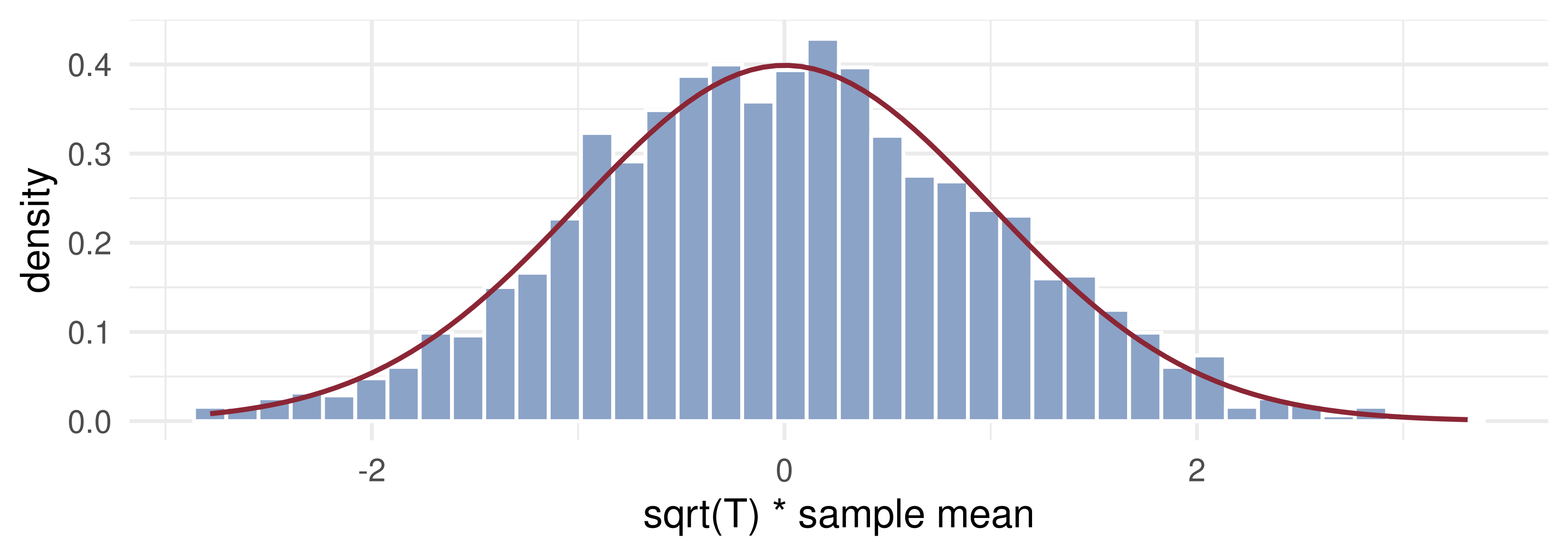
💻 The MDS CLT at Work: ARCH Errors

set.seed(2026)
R <- 2000; T_len <- 500                       # 2000 samples of length 500
x <- matrix(0, T_len, R); prev <- rep(0, R)
for (t in 1:T_len) {                          # ARCH(1): sigma_t^2 = 0.5 + 0.5 x_{t-1}^2
  prev <- sqrt(0.5 + 0.5 * prev^2) * rnorm(R); x[t, ] <- prev }
z <- sqrt(T_len) * colMeans(x)                # sqrt(T) * xbar, one per sample
kurt <- mean(x^4) / mean(x^2)^2               # kurtosis of x_t (3 for a normal)
ggplot(data.frame(z), aes(z)) +
  geom_histogram(aes(y = after_stat(density)), bins = 40, fill = "#8ba3c7", colour = "white") +
  stat_function(fun = dnorm, colour = "#8b2635", linewidth = 1.2) +
  labs(x = "sqrt(T) * sample mean", y = "density") + theme_minimal(base_size = 20)

Each \(x_t\) is fat-tailed (kurtosis 7.5, against 3 for a normal) and dependent through its variance, yet \(\sqrt T\,\bar x_T\) has variance 0.99 and matches \(N(0, \operatorname{Var}x_t) = N(0,1)\) (red).

📐 The General CLT and the Long-Run Variance

Drop the MDS assumption: now \(x_t\) may be correlated with its past.

CLT for S&E sequences (Gordin; under suitable dependence and moment conditions)

\[\frac{1}{\sqrt T}\sum_{t=1}^{T}\big(x_t - E x_t\big) \xrightarrow{d} N(0, V_x), \qquad V_x = \sum_{j=-\infty}^{+\infty}\Gamma_j, \quad \Gamma_j = \operatorname{cov}(x_t, x_{t+j}).\]

\(V_x\) is the long-run variance of \(x_t\). For vector series \(\Gamma_j\) is a matrix and \(\Gamma_{-j} = \Gamma_j^{\top}\). For an MDS, \(\Gamma_j = 0\) for \(j \neq 0\) and \(V_x = \Gamma_0\): the previous theorem is a special case.

🧮 Where \(V_x\) Comes From

Expand the variance of the scaled sum. It is the sum of all \(T^2\) entries of the matrix \(\big(\operatorname{cov}(x_s, x_t)\big)_{s,t}\), and by stationarity the entry depends on \(t - s\) only: \[\begin{aligned}\operatorname{var}\Big(\frac{1}{\sqrt T}\sum_{t=1}^{T}x_t\Big) = \operatorname{var}(x_t) &+ \tfrac{T-1}{T}\big[\operatorname{cov}(x_t, x_{t+1}) + \operatorname{cov}(x_t, x_{t-1})\big] + \tfrac{T-2}{T}\big[\cdots\big] \\ &+ \dots + \tfrac1T\big[\operatorname{cov}(x_1, x_T) + \operatorname{cov}(x_T, x_1)\big].\end{aligned}\]

The \(j\)-th diagonal of the matrix has \(T - |j|\) entries, each equal to \(\Gamma_j\). Hence \[\operatorname{var}\Big(\frac{1}{\sqrt T}\sum_{t=1}^{T}x_t\Big) = \sum_{|j|<T}\Big(1 - \frac{|j|}{T}\Big)\Gamma_j \ \xrightarrow[T\to\infty]{}\ \sum_{j=-\infty}^{\infty}\Gamma_j = V_x,\] provided \(\sum_j|\Gamma_j| < \infty\). Memory enters the variance through every off-diagonal term.

🧮 Worked Example: AR(1) and MA(1)

AR(1), \(x_t = \rho x_{t-1} + \varepsilon_t\): from Lecture 1, \(\Gamma_j = \rho^{|j|}\Gamma_0\) with \(\Gamma_0 = \sigma^2/(1-\rho^2)\). A geometric series: \[V_x = \Gamma_0\Big(1 + 2\sum_{j=1}^{\infty}\rho^j\Big) = \Gamma_0\,\frac{1+\rho}{1-\rho} = \frac{\sigma^2}{(1-\rho)^2}.\]

\(\rho\)	0	0.5	0.8	0.9	0.95
\(V_x/\Gamma_0 = (1+\rho)/(1-\rho)\)	1	3	9	19	39

At \(\rho = 0.9\) the i.i.d. standard error is too small by a factor \(\sqrt{19} \approx 4.4\).

MA(1), \(x_t = \varepsilon_t + \theta\varepsilon_{t-1}\): \(V_x = (1+\theta^2)\sigma^2 + 2\theta\sigma^2 = (1+\theta)^2\sigma^2\). Negative \(\theta\) makes \(V_x < \Gamma_0\).

💻 Two Candidate Variances, One Truth

set.seed(2026)
R <- 2000; T_len <- 500; rho <- 0.8
x <- matrix(0, T_len, R); prev <- rnorm(R, sd = 1 / sqrt(1 - rho^2))  # stationary start
for (t in 1:T_len) { prev <- rho * prev + rnorm(R); x[t, ] <- prev }
z <- sqrt(T_len) * colMeans(x)
ggplot(data.frame(z), aes(z)) +
  geom_histogram(aes(y = after_stat(density)), bins = 40, fill = "#8ba3c7", colour = "white") +
  stat_function(fun = dnorm, args = list(sd = sqrt(1 / (1 - rho^2))), aes(colour = "N(0, Gamma0)"), linewidth = 1.2) +
  stat_function(fun = dnorm, args = list(sd = 1 / (1 - rho)), aes(colour = "N(0, V)"), linewidth = 1.2) +
  scale_colour_manual(values = c("#e09f3e", "#8b2635"), name = NULL) +
  labs(x = "sqrt(T) * sample mean", y = "density") + theme_minimal(base_size = 20) + theme(legend.position = "top")

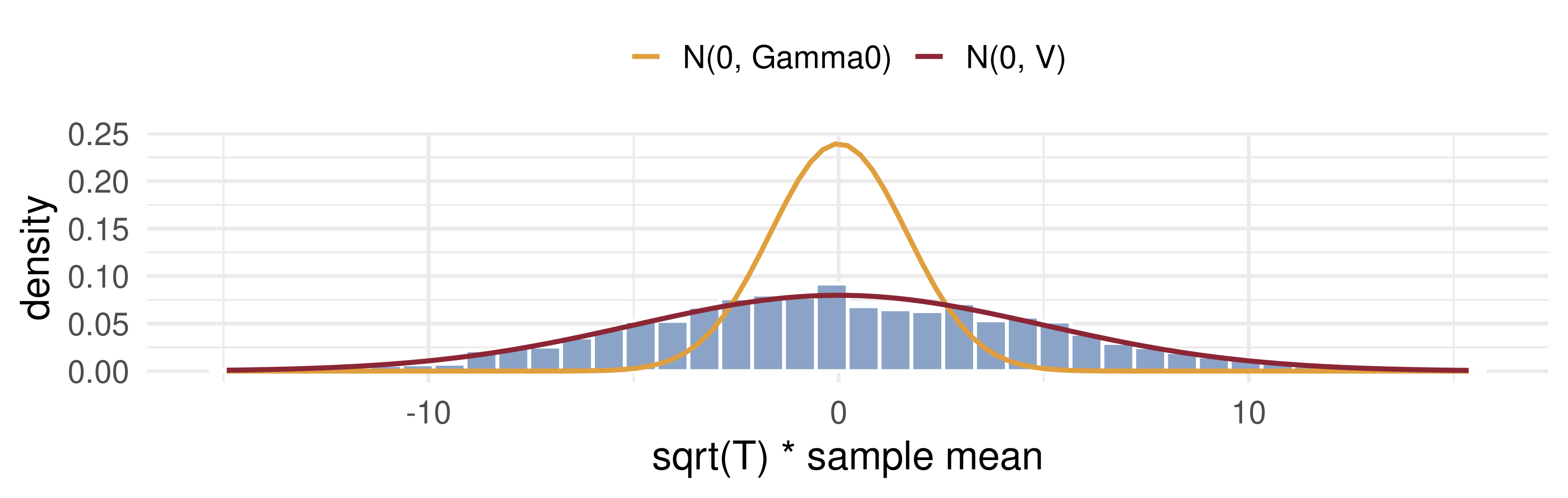
AR(1), \(\rho = 0.8\): \(\Gamma_0 = 2.78\), \(V_x = 25\). Across 2000 samples, \(\operatorname{Var}(\sqrt T\,\bar x_T) =\) 24.7. The long-run variance is the truth; the i.i.d. curve has a ninth of the right variance.

📐 Estimating \(V_x\): Sample Autocovariances

\(V_x\) is a sum of population autocovariances. The natural ingredients are their sample versions (HAC estimation: heteroskedasticity and autocorrelation consistent): \[\hat\Gamma_j = \frac1T\sum_{t=1}^{T-j}(x_t - \bar x)(x_{t+j} - \bar x)^{\top}, \quad j \ge 0, \qquad \hat\Gamma_{-j} = \hat\Gamma_j^{\top}.\]

• Each \(\hat\Gamma_j\) uses only \(T - |j|\) products, yet divides by \(T\).
• \(\hat\Gamma_1\) rests on \(T-1\) pairs and is precise. \(\hat\Gamma_{T-1}\) rests on one pair, \((x_1 - \bar x)(x_T - \bar x)\), and is pure noise.

⚠️ The Naive Estimator Fails

Plug in all of them: \[\hat V_x^{N} = \sum_{j=-(T-1)}^{T-1}\hat\Gamma_j.\]

It is not consistent: the high-order \(\hat\Gamma_j\) are too noisy at the ends, and there are as many of them as observations. In fact it fails in the sharpest possible way. Writing \(u_t = x_t - \bar x\), \[\sum_{|j|<T}\hat\Gamma_j = \frac1T\sum_{s=1}^{T}\sum_{t=1}^{T}u_s u_t^{\top} = \frac1T\Big(\sum_{t}u_t\Big)\Big(\sum_{t}u_t\Big)^{\top} = 0,\] because deviations from the sample mean sum to zero. The naive estimator is identically zero.

The cure is to truncate and down-weight the distant autocovariances.

📐 Newey–West (1987)

Newey–West estimator

\[\hat V_x^{NW} = \sum_{j=-m}^{m}\Big(1 - \frac{|j|}{m+1}\Big)\hat\Gamma_j.\] If \(m \to \infty\) as \(T \to \infty\), but slowly enough that \(m/T \to 0\), then \(\hat V_x^{NW} \xrightarrow{p} V_x\).

• The weights are triangular (Bartlett): 1 at \(j = 0\), falling linearly to 0 at \(j = \pm(m+1)\). They make \(\hat V^{NW}\) positive semi-definite in every sample.
• Rule of thumb (Newey–West, 1994): \(m = \lfloor 4(T/100)^{2/9}\rfloor\), so \(m = 5\) for \(T = 500\). The MSE-optimal rate is \(m \propto T^{1/3}\) (Andrews, 1991).
• For persistent series a fixed rule works poorly: much of \(V_x\) sits beyond lag \(m\).

🔺 Why the Triangle?

Apply the variance-of-a-sum identity to a block of \(n = m+1\) consecutive observations: \[\operatorname{var}\Big(\frac{1}{\sqrt{m+1}}\sum_{i=1}^{m+1}x_{t+i}\Big) = \sum_{|j|\le m}\Big(1 - \frac{|j|}{m+1}\Big)\Gamma_j.\]

The Newey–West weights are exactly the weights that appear in the variance of a block sum. So \(\hat V^{NW}\) is, up to end effects, the average squared scaled block sum of the demeaned data — an average of squares, which cannot be negative.

• Small \(m\): short blocks miss distant autocorrelation, so \(\hat V^{NW}\) is biased toward \(\Gamma_0\).
• Large \(m\): few effectively independent blocks, so \(\hat V^{NW}\) is noisy.
• \(m \to \infty\) with \(m/T \to 0\) balances the two.

📐 Generalisation: Andrews (1991) Kernel Estimators

Kernel HAC estimator

\[\hat V^{A} = \sum_{j=-(T-1)}^{T-1}w(j)\,\hat\Gamma_j, \qquad w(j) = K\Big(\frac{j}{\delta}\Big).\]

• \(K\) is the kernel, \(\delta\) the bandwidth.
• Consistency conditions: \(\delta \to \infty\) and \(\delta/T \to 0\) as \(T \to \infty\); \(K\) is symmetric, continuous at 0 with \(K(0) = 1\), and \(\int_{-\infty}^{\infty}K(u)^2\,du < \infty\).
• Newey–West is the Bartlett kernel with \(\delta = m+1\).

📋 Four Kernels

Kernel	\(K(u)\)	Consistent	PSD in every sample
Uniform	\(1\) for \(\lvert u\rvert \le 1\); 0 otherwise	yes	no
Bartlett (Newey–West)	\(1 - \lvert u\rvert\) for \(\lvert u\rvert \le 1\); 0 otherwise	yes	yes
Parzen	\(1 - 6u^2 + 6\lvert u\rvert^3\) for \(\lvert u\rvert \le \frac12\); \(\ 2(1-\lvert u\rvert)^3\) for \(\frac12 \le \lvert u\rvert \le 1\)	yes	yes
Quadratic spectral	\(\dfrac{25}{12\pi^2u^2}\Big(\dfrac{\sin(6\pi u/5)}{6\pi u/5} - \cos(6\pi u/5)\Big)\)	yes	yes

Uniform: \(\hat V = \sum_{|j|\le\delta}\hat\Gamma_j\), consistent but possibly negative in a sample. QS is never exactly zero: every \(\hat\Gamma_j\) gets some weight.

🎛️ Explore: Kernel Weights

viewof delta = Inputs.range([2, 30], {step: 1, value: 10, label: "Bandwidth δ"})

kern = {
  const qs = u => { if (u === 0) return 1; const a = 6 * Math.PI * u / 5;
    return 25 / (12 * Math.PI * Math.PI * u * u) * (Math.sin(a) / a - Math.cos(a)); };
  const K = {
    "Uniform": u => Math.abs(u) <= 1 ? 1 : 0,
    "Bartlett": u => Math.abs(u) <= 1 ? 1 - Math.abs(u) : 0,
    "Parzen": u => { const a = Math.abs(u);
      return a <= 0.5 ? 1 - 6 * a * a + 6 * a ** 3 : (a <= 1 ? 2 * (1 - a) ** 3 : 0); },
    "Quadratic spectral": qs };
  const out = [];
  for (const name of Object.keys(K))
    for (let j = 0; j <= 40; j++) out.push({lag: j, w: K[name](j / delta), kernel: name});
  return out;
}

Plot.plot({
  width: 1100, height: 300, marginLeft: 78, marginBottom: 50,
  style: {fontSize: "18px"},
  x: {label: "lag j", domain: [0, 40]}, y: {label: "weight w(j)", domain: [-0.15, 1.05], grid: true},
  color: {domain: ["Uniform", "Bartlett", "Parzen", "Quadratic spectral"],
          range: ["#9a9a9a", "#2f4b7c", "#e09f3e", "#8b2635"]},
  marks: [
    Plot.ruleY([0]),
    Plot.line(kern, {x: "lag", y: "w", stroke: "kernel", strokeWidth: 3, curve: "step-after", filter: d => d.kernel === "Uniform"}),
    Plot.line(kern, {x: "lag", y: "w", stroke: "kernel", strokeWidth: 3, filter: d => d.kernel !== "Uniform"})
  ]
})

Grey: uniform, blue: Bartlett, amber: Parzen, red: QS. Larger \(\delta\) stretches every kernel over more lags; only QS dips below zero and never quite stops.

🪶 Why Smoothness Matters

• Bartlett falls linearly from \(u = 0\): even \(\hat\Gamma_1\) is down-weighted by \(1/\delta\). Its weights converge to 1 slowly as \(\delta\) grows, so its bias shrinks slowly.
• Parzen and QS are flat at the top, \(K(u) = 1 - O(u^2)\): low-order autocovariances, the precisely estimated ones, get weight close to 1. Their bias shrinks faster.

Kernel	bias of order	MSE-optimal bandwidth
Bartlett	\(\delta^{-1}\)	\(\delta \propto T^{1/3}\)
Parzen, QS	\(\delta^{-2}\)	\(\delta \propto T^{1/5}\)

QS minimises the asymptotic MSE among kernels that guarantee a PSD estimate (Andrews, 1991). For smoothness, Parzen is preferred to Bartlett.

💻 Newey–West Converges, Slowly

set.seed(2026)
nw <- function(x, m) { u <- x - mean(x); n <- length(u)
  g <- sapply(0:m, function(j) sum(u[1:(n - j)] * u[(1 + j):n]) / n)
  g[1] + 2 * sum((1 - (1:m) / (m + 1)) * g[-1]) }
rho <- 0.5; V_true <- 1 / (1 - rho)^2                  # = 4, while Gamma0 = 1.33
sims <- do.call(rbind, lapply(c(200, 1000, 5000), function(n) {
  rules <- c(`4(T/100)^(2/9)` = floor(4 * (n / 100)^(2 / 9)), `T^(1/3)` = floor(n^(1 / 3)))
  do.call(rbind, lapply(names(rules), function(r) data.frame(T = factor(n), rule = r,
    V = replicate(300, nw(as.numeric(filter(rnorm(n), rho, "recursive")), rules[[r]])))))
}))
ggplot(sims, aes(T, V, fill = rule)) + geom_boxplot(outlier.size = 0.6) +
  geom_hline(yintercept = V_true, colour = "#8b2635", linewidth = 1.1) +
  scale_fill_manual(values = c("#8ba3c7", "#e09f3e"), name = "lag rule") +
  labs(x = "sample size T", y = expression(hat(V)^NW)) + theme(legend.position = "top")

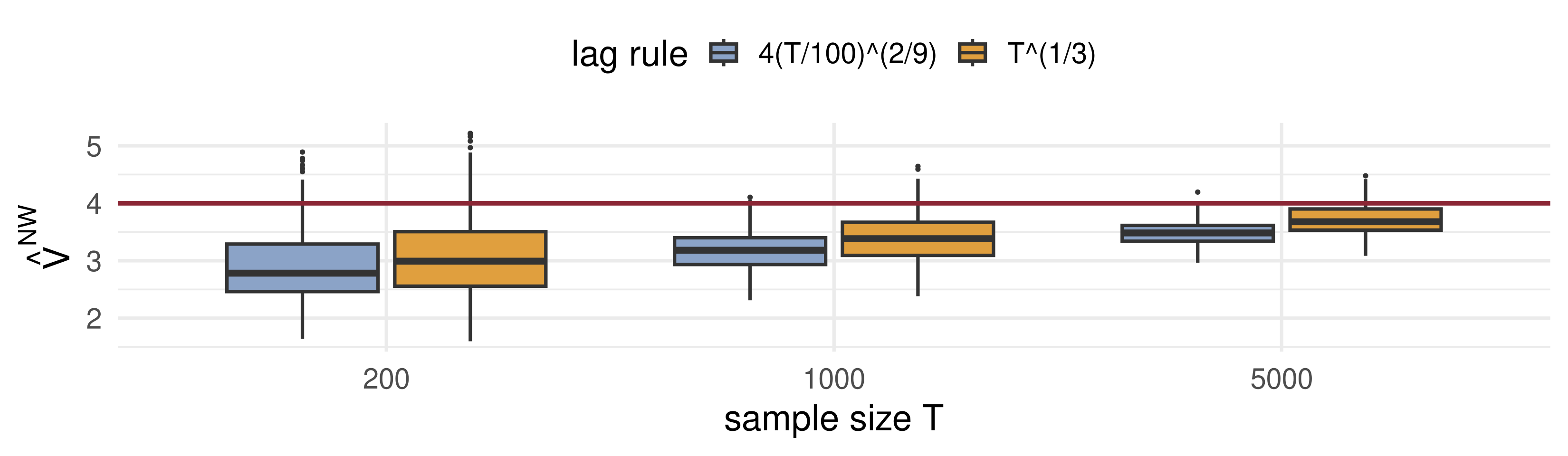
AR(1), \(\rho = 0.5\), true \(V_x = 4\) (red). The boxes tighten and climb toward 4, but at \(T = 5000\) both rules are still biased down: the price of the triangle.

🧠 Think–Pair–Share

A daily trading strategy’s P&L follows \(x_t = \varepsilon_t - 0.5\,\varepsilon_{t-1}\), with \(\varepsilon_t\) i.i.d., \(\operatorname{Var}\varepsilon_t = 1\) (a bid–ask bounce).

1. Compute \(\Gamma_0\), \(\Gamma_1\) and the long-run variance \(V_x\).
2. Is the i.i.d. standard error of \(\bar x_T\) too large or too small, and by what factor?
3. In population, what does Newey–West with \(m = 1\) give? And the uniform kernel with \(\delta = 1\)?

✅ Think–Pair–Share: Solution

1. \(\Gamma_0 = 1.25\), \(\ \Gamma_1 = \theta\sigma^2 = -0.5\), \(\ \Gamma_j = 0\) for \(|j| \ge 2\). So \(V_x = 1.25 - 1 = 0.25 = (1+\theta)^2\).

2. Too large, by \(\sqrt{\Gamma_0/V_x} = \sqrt5 \approx 2.24\). Negative autocorrelation makes the average more precise.

3. Newey–West, \(m = 1\): \(\ \Gamma_0 + 2\cdot\tfrac12\Gamma_1 = 0.75\), three times too large, though the memory ends at lag 1: the triangle halves \(\Gamma_1\). The uniform kernel with \(\delta = 1\) gives \(\Gamma_0 + 2\Gamma_1 = 0.25\) exactly, but in a sample \(\hat\Gamma_0 + 2\hat\Gamma_1\) can be negative.

💰 Case Study: Average Inflation

📈 The question

What is the standard error of average US inflation since 1985?

1. How far apart are the i.i.d. variance \(\hat\Gamma_0\) and the long-run variance \(\hat V\)?
2. Does \(\hat V^{NW}\) settle as the truncation lag \(m\) grows?
3. Do Parzen and QS kernels tell the same story?

📊 The data

Series: CPI for all urban consumers, seasonally adjusted (FRED CPIAUCSL)

Period: Jan 1985 – Sep 2026, \(T = 501\) months

Transformation: \(\pi_t = 1200\,(\log P_t - \log P_{t-1})\), annualised %

# How the file was obtained (not run)
download.file(paste0(
  "https://fred.stlouisfed.org/graph/",
  "fredgraph.csv?id=CPIAUCSL"),
  "data/CPIAUCSL.csv")

💰 Case Study: Long-Run Variances in R

cpi <- read.csv("data/CPIAUCSL.csv")
lp <- log(cpi$CPIAUCSL)
gap <- which(is.na(lp)); lp[gap] <- (lp[gap - 1] + lp[gap + 1]) / 2   # Oct 2025 not published: interpolate
infl <- 1200 * diff(lp); n <- length(infl); u <- infl - mean(infl)
G <- sapply(0:(n - 1), function(j) sum(u[1:(n - j)] * u[(1 + j):n]) / n)      # Gamma-hat_0 ... _{T-1}
K <- list(bartlett = function(x) pmax(1 - abs(x), 0),
          parzen = function(x) { a <- abs(x); ifelse(a <= .5, 1 - 6*a^2 + 6*a^3, ifelse(a <= 1, 2*(1 - a)^3, 0)) },
          qs = function(x) { a <- 6*pi*x/5; ifelse(x == 0, 1, 25/(12*pi^2*x^2) * (sin(a)/a - cos(a))) })
Vhat <- function(k, d) G[1] + 2 * sum(K[[k]]((1:(n - 1)) / d) * G[-1])
m_rule <- floor(4 * (n / 100)^(2 / 9))
V <- c(Gamma0 = G[1], naive = G[1] + 2 * sum(G[-1]), NW_rule = Vhat("bartlett", m_rule + 1),
       NW_m12 = Vhat("bartlett", 13), NW_m36 = Vhat("bartlett", 37), Parzen_d12 = Vhat("parzen", 12), QS_d12 = Vhat("qs", 12))
round(rbind(V = V, se_of_mean = sqrt(pmax(V, 0) / n)), 3)

           Gamma0 naive NW_rule NW_m12 NW_m36 Parzen_d12 QS_d12
V          10.206     0  20.971 28.242 40.621     24.628 30.381
se_of_mean  0.143     0   0.205  0.237  0.285      0.222  0.246

Mean inflation is 2.78% and the rule-of-thumb lag is \(m =\) 5. Compare the standard errors along the bottom row.

💰 Case Study: Estimates vs Bandwidth

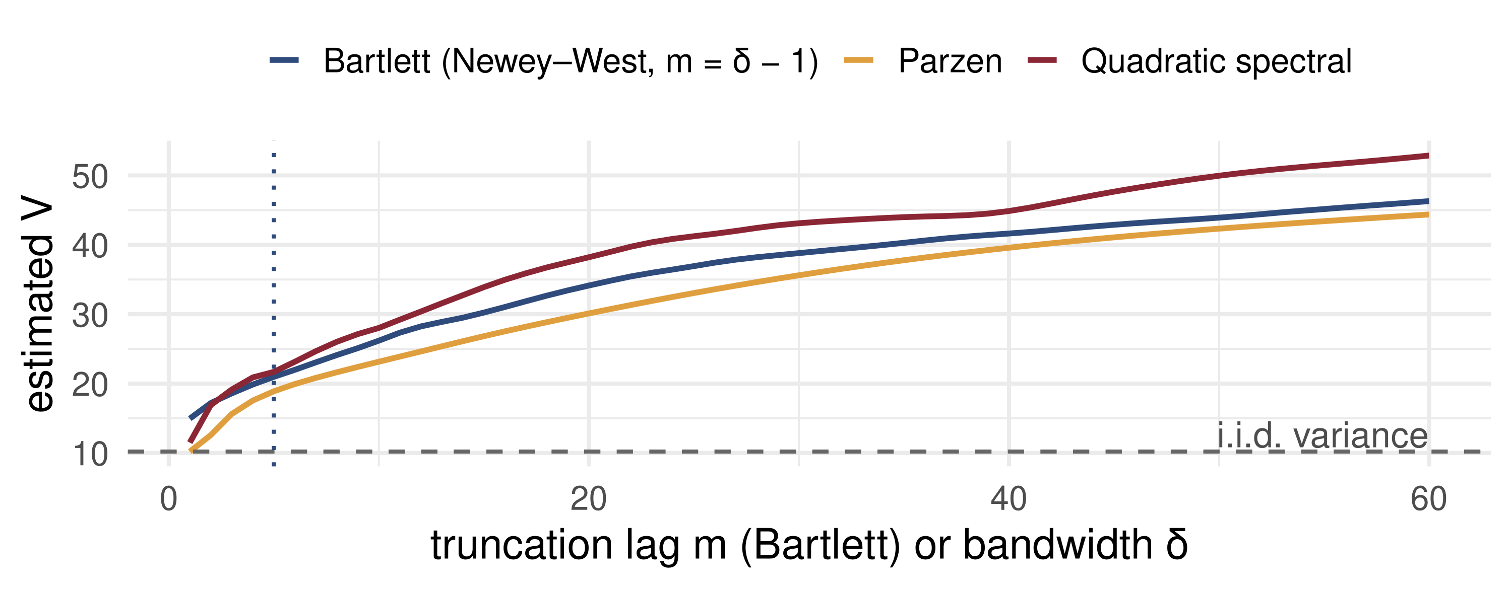
What the data say: every HAC estimate lies far above \(\hat\Gamma_0 \approx 10\), so the i.i.d. standard error (\(0.14\)) understates the uncertainty; at the rule-of-thumb lag (\(m = 5\), dotted) it is about \(0.20\). But no curve settles: \(\hat V\) keeps rising with \(m\), because inflation’s autocorrelations stay small and positive for years. For a series this persistent the fixed rule is not enough, exactly the warning of the theory.

📝 Quiz #1: The Long-Run Variance

\(x_t = 0.75\,x_{t-1} + \varepsilon_t\), \(\operatorname{Var}\varepsilon_t = 1\). What is the long-run variance \(V_x\)?

• \(1/(1 - 0.75^2) \approx 2.29\)
• \(1\)
• \(1/(1 - 0.75)^2 = 16\)
• \((1 + 0.75)^2 = 3.06\)

📝 Quiz #2: The Naive Estimator

Why is \(\hat V^{N} = \sum_{j=-(T-1)}^{T-1}\hat\Gamma_j\) useless?

• It is consistent but not positive semi-definite
• It needs the true mean \(E x_t\), which is unknown
• With the sample mean subtracted, it equals zero in every sample
• It ignores \(\hat\Gamma_0\)

📝 Quiz #3: Bandwidth Rates

For the Newey–West estimator to be consistent, the truncation lag \(m\) must satisfy …

• \(m\) fixed, e.g. \(m = 5\), whatever \(T\)
• \(m = T - 1\), to use every autocovariance
• \(m \to \infty\) and \(m/T \to 0\) as \(T \to \infty\)
• \(m/T \to 1/2\)

📋 Key Formulas

Ergodic theorem	\(\bar x_T \xrightarrow{p} E x_t\) for S&E \(x_t\), \(E\lvert x_t\rvert < \infty\)
CLT, S&E MDS	\(T^{-1/2}\sum x_t \xrightarrow{d} N(0, \operatorname{Var}x_t)\)
CLT, S&E	\(T^{-1/2}\sum (x_t - Ex_t) \xrightarrow{d} N(0, V_x)\), \(\ V_x = \sum_{j}\Gamma_j\)
Finite-\(T\) variance	\(\operatorname{var}(T^{-1/2}\sum x_t) = \sum_{\lvert j\rvert<T}(1 - \lvert j\rvert/T)\Gamma_j\)
AR(1) / MA(1)	\(V_x = \sigma^2/(1-\rho)^2\) / \(V_x = (1+\theta)^2\sigma^2\)
Newey–West	\(\hat V^{NW} = \sum_{\lvert j\rvert\le m}(1 - \lvert j\rvert/(m+1))\hat\Gamma_j\), \(\ m = \lfloor 4(T/100)^{2/9}\rfloor\)
Andrews	\(\hat V^{A} = \sum_{\lvert j\rvert<T}K(j/\delta)\hat\Gamma_j\), \(\ \delta\to\infty\), \(\delta/T\to0\)

📋 Summary

• The ergodic theorem needs both S and E; the random walk’s mean has variance of order \(T\)
• For an S&E martingale difference sequence, the CLT holds with the ordinary variance — no independence needed
• With serial correlation the CLT variance is the long-run variance \(V_x = \sum_j\Gamma_j\), often many times \(\Gamma_0\)
• Plugging in all sample autocovariances gives exactly zero; truncation and down-weighting fix it
• Newey–West uses triangular weights, which keep \(\hat V\) non-negative; smoother kernels (Parzen, QS) have smaller bias
• Bandwidths must grow, but slower than \(T\); for persistent series, fixed rules are not enough

📚 Further Reading

• Hamilton, J. D. (1994). Time Series Analysis, ch. 7 (limit theorems for dependent data) and §10.5 (the long-run variance, Newey–West).
• Hayashi, F. (2000). Econometrics, §2.2 and §6.6 (ergodic theorem, MDS CLT, HAC estimation).
• Newey, W. K. and West, K. D. (1987). A simple, positive semi-definite, heteroskedasticity and autocorrelation consistent covariance matrix. Econometrica 55, 703–708.
• Andrews, D. W. K. (1991). Heteroskedasticity and autocorrelation consistent covariance matrix estimation. Econometrica 59, 817–858.
• Newey, W. K. and West, K. D. (1994). Automatic lag selection in covariance matrix estimation. Review of Economic Studies 61, 631–653.

Next lecture: Time-Series Regression and HAC Inference — the same long-run variance, now inside the OLS sandwich.