Time Series Econometrics

Lecture 3: Time-Series Regression and HAC Inference

Samir Orujov, PhD

Open lecture notes, after Stanislav Anatolyev’s course (2016)

🎬 The Idea in 3 Minutes

⬅ Previous lecture: 2 · Ergodic Theorem, CLT and the Long-Run Variance

A short film with the intuition. Watch it before the slides, or after. Captions: CC button.

🎯 Learning Objectives

By the end of this lecture, you will be able to:

Derive the asymptotic distribution of OLS with stationary ergodic data, and recognise the long-run variance inside the sandwich
Decide when ordinary or White standard errors suffice and when HAC standard errors are needed
Show that overlapping forecast horizons make regression errors MA(\(h-1\)), and choose the truncation lag accordingly
Compute OLS, White and Newey–West standard errors by hand in R for Mishkin’s inflation regression
Distinguish structural from non-structural time-series modelling

🔁 Warm-up from last time

\(x_t\) is a stationary ergodic martingale difference sequence with \(\operatorname{Var}x_t = \sigma^2\). What is its long-run variance \(V_x = \sum_j\Gamma_j\)?

\(\sigma^2/(1-\rho)^2\) for some persistence \(\rho\)
\(\sigma^2\), the same as its ordinary variance
\(0\), because the naive estimator is identically zero
It cannot be determined without a kernel and a bandwidth

🗺️ Where We Are

Lecture 2 ended with the long-run variance \(V_x = \sum_j\Gamma_j\) and its kernel estimators: truncate, down-weight, let the bandwidth grow slowly.

We used it for a single mean. Today the same object appears in regression. The OLS estimator is a ratio of two sample averages; the denominator obeys the ergodic theorem, the numerator obeys the CLT, and its variance is the long-run variance of \(x_t\varepsilon_t\).

The practical question becomes: when is \(x_t\varepsilon_t\) an MDS, so that the simple formulas are right, and when do we need HAC?

❓ The Question

Does the T-bill rate know future inflation?

The Fisher equation says the nominal rate is a real rate plus expected inflation, \(i_t = r + E_t\pi\). If the real rate is roughly stable, today’s 3-month Treasury-bill rate should forecast inflation over the next three months.

Mishkin (1990) tested this by regressing future inflation on today’s interest rate. The point estimate is easy. The standard error is not: with monthly data and a three-month horizon, consecutive forecast errors overlap, and the textbook OLS standard error is wrong.

📐 Time-Series Regression

\[y_t = x_t'\beta + \varepsilon_t, \qquad t = 1, \dots, T.\]

Assumptions

\((y_t, x_t)\) is strictly stationary and ergodic;
\(E(\varepsilon_t \mid x_t, x_{t-1}, \dots) = 0\): the error is unpredictable from current and past regressors (at the least, \(E(x_t\varepsilon_t) = 0\));
\(Q = E(x_tx_t')\) is non-singular.

Then OLS is applicable: it is consistent and asymptotically normal. Its standard errors must sometimes be HAC — when \(x_t\varepsilon_t\) is serially correlated. When it is not, they need not be.

🧮 OLS Asymptotics, Step by Step

Substitute \(y_t = x_t'\beta + \varepsilon_t\) into \(\hat\beta = (X'X)^{-1}X'y\): \[\sqrt T(\hat\beta - \beta) = \Big(\frac1T\sum_{t=1}^{T}x_tx_t'\Big)^{-1}\ \frac{1}{\sqrt T}\sum_{t=1}^{T}x_t\varepsilon_t.\]

Denominator. \(x_tx_t'\) is a function of an S&E series, hence S&E (Lecture 1). Ergodic theorem: \(\frac1T\sum x_tx_t' \xrightarrow{p} Q\).
Numerator. \(g_t = x_t\varepsilon_t\) is S&E with mean zero. CLT (Lecture 2): \(T^{-1/2}\sum g_t \xrightarrow{d} N(0, V)\), where \(V = \sum_j\Gamma_j(g)\) is the long-run variance of \(x_t\varepsilon_t\).

Combine them (Slutsky): \[\sqrt T(\hat\beta - \beta) \xrightarrow{d} N\big(0,\ Q^{-1}VQ^{-1}\big).\] The “sandwich”: \(Q^{-1}\) is the bread, the long-run variance \(V\) the filling.

📐 When Is HAC Not Needed?

Suppose the error is an MDS with respect to everything dated \(t\) and earlier, regressors included: \[E(\varepsilon_t \mid x_t, x_{t-1}, \dots,\ \varepsilon_{t-1}, \varepsilon_{t-2}, \dots) = 0.\]

Then \(g_t = x_t\varepsilon_t\) is an MDS too. For \(j \ge 1\), everything in \(g_{t-j}\) and \(x_t\) is in the conditioning set, so \[E(g_tg_{t-j}') = E\big[x_t\,E(\varepsilon_t \mid \dots)\,g_{t-j}'\big] = 0.\] Only \(\Gamma_0(g) = E(\varepsilon_t^2x_tx_t')\) survives: the short-run variance.

\(V = E(\varepsilon_t^2x_tx_t')\): White (heteroskedasticity-robust) standard errors.
If also \(E(\varepsilon_t^2 \mid x_t) = \sigma^2\): \(V = \sigma^2Q\), and the classical \(\sigma^2(X'X)^{-1}\) is right.
If \(\varepsilon_t\) is predictable from its own past (overlap, omitted dynamics): \(\Gamma_j(g) \ne 0\), and we need HAC.

📐 The HAC Variance of OLS

With residuals \(\hat e_t = y_t - x_t'\hat\beta\): \[\hat V_{OLS} = \Big(\frac{X'X}{T}\Big)^{-1}\ \hat V_{HAC}\ \Big(\frac{X'X}{T}\Big)^{-1}, \qquad \hat V_{HAC} = \sum_{j=-(T-1)}^{T-1}K\Big(\frac{j}{\delta}\Big)\hat\Gamma_j(x_t\hat e_t),\] \[\hat\Gamma_j(x_t\hat e_t) = \frac1T\sum_{t=1}^{T-j}\hat e_t\,\hat e_{t+j}\,x_t\,x_{t+j}', \quad j \ge 0, \qquad \hat\Gamma_{-j} = \hat\Gamma_j'.\]

\(\hat V_{OLS}\) estimates the variance of \(\sqrt T(\hat\beta - \beta)\), so \(\widehat{\operatorname{Var}}(\hat\beta) = \hat V_{OLS}/T\).
The kernel weights are essential. Without them, \(\sum_{|j|<T}\hat\Gamma_j(x_t\hat e_t) = \frac1T\big(\sum_t x_t\hat e_t\big)\big(\sum_t x_t\hat e_t\big)' = 0\), since the OLS normal equations give \(\sum_t x_t\hat e_t = 0\): the naive estimator again.
With the Bartlett kernel and \(\delta = m+1\), this is the Newey–West estimator.

🏦 Mishkin I: One-Month Horizon

Predict next month’s inflation by this month’s one-month interest rate \(i_t\): \[\pi_{t+1} = \alpha + \beta\,i_t + e_{t+1}, \qquad E(e_{t+1} \mid i_t, i_{t-1}, \dots, \pi_t, \pi_{t-1}, \dots) = 0.\]

\(H_0: \beta = 0\): \(i_t\) carries no information about future inflation.
\(H_0: \alpha = 0,\ \beta = 1\): \(i_t\) is an unbiased predictor of inflation.

The error is an MDS with respect to the information at \(t\), which contains \(e_t, e_{t-1}, \dots\). So it is serially uncorrelated: HAC is not necessary; the short-run variance (White) suffices.

🏦 Mishkin II: Three-Month Horizon

With monthly data, predict inflation over the next three months by the three-month rate \(i_{t,3}\): \[\pi_{t,3} = \alpha + \beta\,i_{t,3} + e_{t+3}, \qquad E\big[e_{t+3} \mid i_{t,3}, \pi_t, \pi_{t-1}, \dots\big] = 0.\]

The error is unpredictable at \(t\), but it is not known until \(t+3\). Let \(\eta_{s}\) be the inflation news that arrives in month \(s\) (an MDS). Then, roughly, \[e_{t+3} = \eta_{t+1} + \eta_{t+2} + \eta_{t+3}, \qquad e_{t+4} = \eta_{t+2} + \eta_{t+3} + \eta_{t+4}.\] Neighbouring errors share two months of news; errors two months apart share one; three apart, none.

So \(e_{t+3}\) is MA(2). OLS is still consistent, since \(E(i_{t,3}e_{t+3}) = 0\), but HAC is needed, with truncation lag at least 2.

🧮 Worked Example: How Wrong Is OLS?

Take \(\operatorname{Var}\eta_s = \sigma^2\) and count shared months: \[\Gamma_0(e) = 3\sigma^2, \quad \Gamma_1(e) = 2\sigma^2, \quad \Gamma_2(e) = \sigma^2, \quad \Gamma_j(e) = 0 \ (j \ge 3).\] Autocorrelations \(\tfrac23, \tfrac13, 0\): a triangle.

For an intercept-only regression: \[V = 3\sigma^2 + 2(2\sigma^2 + \sigma^2) = 9\sigma^2 = 3\,\Gamma_0(e).\] The OLS standard error is too small by \(\sqrt3 \approx 1.73\).

Uniform kernel, \(\delta = 2\): \(\ 3 + 2(2 + 1) = 9\), exact (Hansen and Hodrick, 1980), but not always PSD.
Newey–West, \(m = 2\): \(\ 3 + 2\big(\tfrac23\cdot2 + \tfrac13\cdot1\big) = 6.33\), biased down; Bartlett needs \(m\) well above 2.

🎛️ Explore: The Forecast Horizon

Code

acf_data = {
  const T = 600, rng = d3.randomNormal.source(d3.randomLcg(0.3))(0, 1);
  const eta = Array.from({length: T + h}, () => rng());
  const e = Array.from({length: T}, (_, t) => d3.sum(eta.slice(t, t + h)));
  const m = d3.mean(e), c0 = d3.sum(e, v => (v - m) ** 2);
  const out = [];
  for (let j = 0; j <= 15; j++) {
    let c = 0; for (let t = 0; t < T - j; t++) c += (e[t] - m) * (e[t + j] - m);
    out.push({lag: j, theory: Math.max(1 - j / h, 0), sample: c / c0});
  }
  return out;
}

Bars: theory, \(1 - j/h\) up to lag \(h-1\). Red dots: one simulated sample of \(T = 600\) months. The long-run variance is \(h\) times \(\Gamma_0(e)\): at \(h = 12\) the OLS standard error of a mean is too small by \(\sqrt{12} \approx 3.5\).

💻 Monte Carlo: A True Null

Code

set.seed(2026)
hac_se <- function(X, e, m, uniform = FALSE) {           # sandwich SE, Bartlett or uniform kernel
  n <- nrow(X); g <- X * e; S <- crossprod(g) / n
  for (j in seq_len(m)) { w <- if (uniform) 1 else 1 - j / (m + 1)
    G <- crossprod(g[(1 + j):n, , drop = FALSE], g[1:(n - j), , drop = FALSE]) / n
    S <- S + w * (G + t(G)) }
  Qi <- solve(crossprod(X) / n); sqrt(diag(Qi %*% S %*% Qi) / n) }
n <- 300; R <- 2000
rej <- replicate(R, {
  eta <- rnorm(n + 3); y <- eta[2:(n + 1)] + eta[3:(n + 2)] + eta[4:(n + 3)]   # 3-month overlap, beta = 0
  x <- as.numeric(filter(rnorm(n), 0.95, "recursive")); X <- cbind(1, x)       # persistent "interest rate"
  b <- solve(crossprod(X), crossprod(X, y)); e <- as.numeric(y - X %*% b)
  se <- c(OLS = sqrt(sum(e^2) / (n - 2) * solve(crossprod(X))[2, 2]), White = hac_se(X, e, 0)[[2]],
          `NW m=2` = hac_se(X, e, 2)[[2]], `NW m=5` = hac_se(X, e, 5)[[2]], `Uniform m=2` = hac_se(X, e, 2, TRUE)[[2]])
  abs(b[2] / se) > 1.96 })
rate <- rowMeans(rej, na.rm = TRUE)
ggplot(data.frame(se = factor(names(rate), names(rate)), rate), aes(se, rate)) +
  geom_col(fill = "#8ba3c7", width = 0.6) + geom_hline(yintercept = 0.05, colour = "#8b2635", linewidth = 1.2) +
  geom_text(aes(label = sprintf("%.1f%%", 100 * rate)), vjust = -0.3, size = 6) +
  scale_y_continuous(labels = scales::percent, limits = c(0, 0.31)) + labs(x = NULL, y = "rejection rate") +
  theme_minimal(base_size = 20)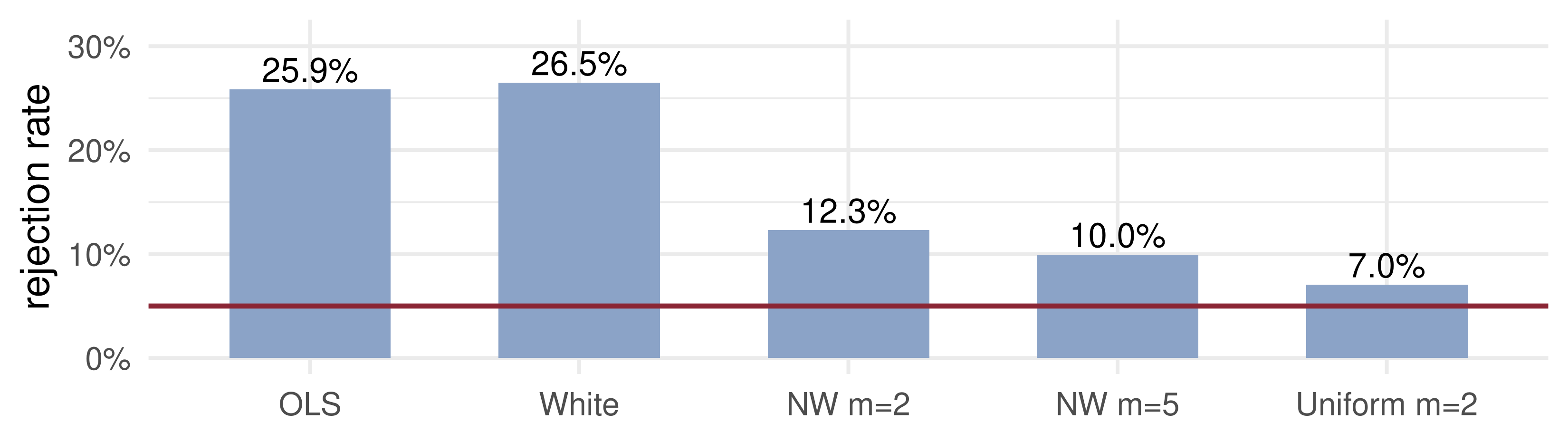

True \(\beta = 0\), nominal size 5% (red). OLS and White reject about a quarter of the time. HAC brings it down; with \(T = 300\) and a persistent regressor it is not yet 5%.

🧠 Think–Pair–Share

A central bank regresses next year’s inflation on today’s one-year rate, using monthly data: \[\pi_{t,12} = \alpha + \beta\,i_{t,12} + e_{t+12}, \qquad E(e_{t+12} \mid \text{information at } t) = 0.\]

What is the MA order of \(e_{t+12}\)? What is the smallest sensible truncation lag?
If the monthly news is i.i.d., by what factor does the OLS standard error of the intercept understate the truth?
Would you use Newey–West with \(m = 11\)? What else?

✅ Think–Pair–Share: Solution

Twelve months of news overlap, so \(e_{t+12}\) is MA(11): \(\Gamma_j(e) \ne 0\) for \(|j| \le 11\), zero beyond. The truncation lag must be at least 11.

\(\Gamma_j(e) = (12 - |j|)\sigma^2\), so \(V = \sum_{|j|\le11}(12-|j|)\sigma^2 = 144\sigma^2 = 12\,\Gamma_0(e)\). The OLS standard error is too small by \(\sqrt{12} \approx 3.5\).

Newey–West with \(m = 11\) is biased down: it weights \(\Gamma_{11}\) by only \(\tfrac1{12}\). Better a larger \(m\), a smoother kernel with a wider bandwidth, or the uniform kernel at 11 (Hansen–Hodrick), checking that the estimate is positive. And 1960–2026 holds only about 66 non-overlapping years, not 790 independent observations.

💰 Case Study: Mishkin Today

📈 The question

Does the 3-month T-bill rate predict inflation over the next three months?

What are \(\hat\alpha\), \(\hat\beta\)?
How much do the OLS, White and Newey–West standard errors differ?
Do the residuals look MA(2), as the theory predicts?

📊 The data

Series: CPI (FRED CPIAUCSL), 3-month T-bill rate (FRED TB3MS)

Period: Jan 1960 – Jun 2026, monthly, \(T = 798\)

Variables: \(\pi_{t,3} = 400\,(\log P_{t+3} - \log P_t)\), annualised %; \(i_{t,3}\) = T-bill rate, %

💰 Case Study: Four Standard Errors

# How the files were obtained (not run)
u <- "https://fred.stlouisfed.org/graph/fredgraph.csv?id="
for (id in c("CPIAUCSL", "TB3MS")) download.file(paste0(u, id), paste0("data/", id, ".csv"))

📦 OLS by hand; OLS, White and Newey–West standard errors

d <- merge(read.csv("data/CPIAUCSL.csv"), read.csv("data/TB3MS.csv"), by = "observation_date")
lp <- log(d$CPIAUCSL); g <- which(is.na(lp)); lp[g] <- (lp[g - 1] + lp[g + 1]) / 2  # Oct 2025 CPI not published
n0 <- nrow(d); pi3 <- 400 * (c(lp[4:n0], rep(NA, 3)) - lp)                           # inflation over t..t+3
dat <- na.omit(data.frame(date = as.Date(d$observation_date), pi3, i = d$TB3MS))
dat <- dat[dat$date >= as.Date("1960-01-01"), ]
X <- cbind(1, dat$i); y <- dat$pi3; n <- nrow(X)
b <- solve(crossprod(X), crossprod(X, y)); e <- as.numeric(y - X %*% b)
se <- cbind(OLS = sqrt(diag(sum(e^2) / (n - 2) * solve(crossprod(X)))), White = hac_se(X, e, 0),
            `NW m=2` = hac_se(X, e, 2), `NW m=12` = hac_se(X, e, 12))
fit <- lm(pi3 ~ i, dat)                                                    # cross-check with sandwich
stopifnot(all.equal(unname(se[, 4]), unname(sqrt(diag(sandwich::NeweyWest(fit, lag = 12, prewhite = FALSE, adjust = FALSE))))))
tab <- rbind(estimate = c(b, NA, NA),
             cbind(t(se), `t(beta=0)` = b[2] / se[2, ], `t(beta=1)` = (b[2] - 1) / se[2, ]))
dimnames(tab) <- list(c("estimate", paste("se", colnames(se))), c("alpha", "beta", "t(beta=0)", "t(beta=1)"))
round(tab, 3)

           alpha  beta t(beta=0) t(beta=1)
estimate   1.384 0.520        NA        NA
se OLS     0.165 0.031    16.918   -15.606
se White   0.183 0.039    13.334   -12.300
se NW m=2  0.290 0.063     8.225    -7.587
se NW m=12 0.448 0.108     4.825    -4.451

💰 Case Study: Are the Errors MA(2)?

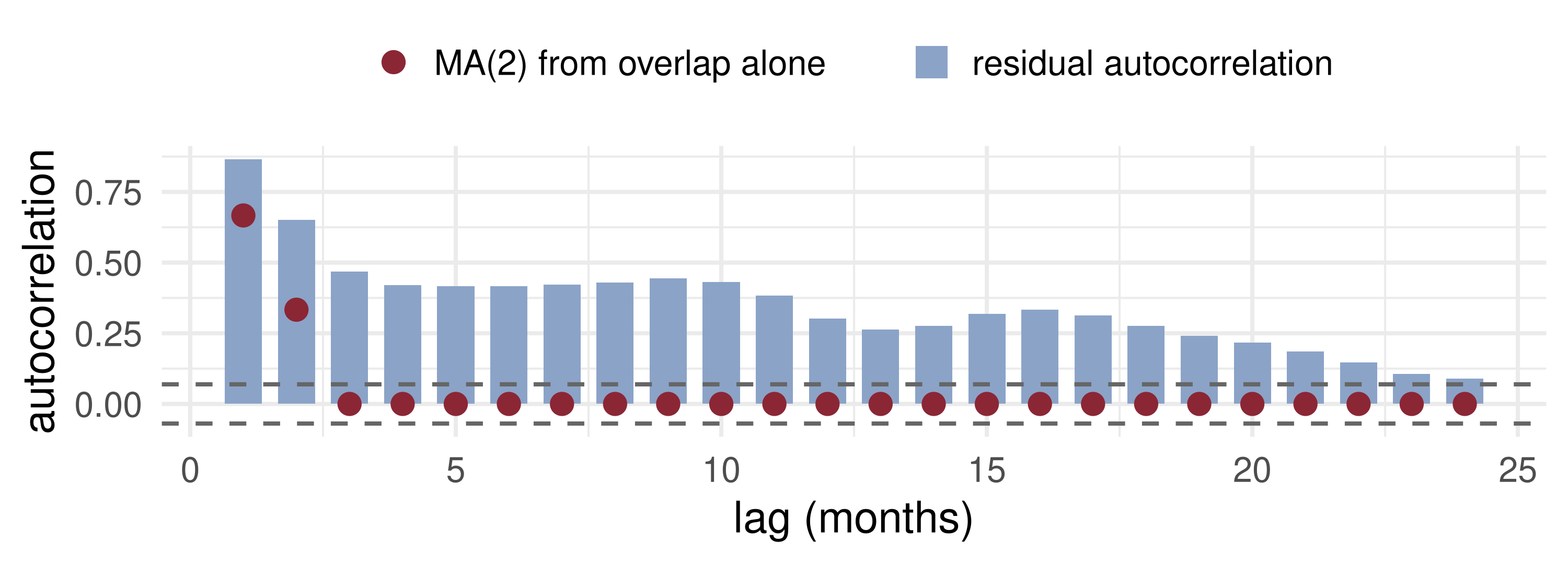
What the data say: \(\hat\beta \approx 0.52\) — the T-bill rate does carry information about inflation (\(\beta = 0\) rejected under every standard error), but it is not an unbiased predictor (\(\beta = 1\) rejected too). The Newey–West standard errors are two (\(m = 2\)) to three and a half (\(m = 12\)) times the OLS ones. The residuals fit MA(2) only at lags 1–2: beyond that they stay near 0.4 for two years. The rate alone leaves predictable, persistent inflation in the error, so even \(m = 12\) may be too short, and a regression with lagged inflation is the better model.

🏛️ Two Ways to Model Time Series

	Structural	Non-structural
Starting point	economic theory, optimally behaving agents	data fit
Goal	estimate and test deep parameters with economic meaning (GMM)	stylised facts; forecasts, dynamics
Example	consumption Euler equation	GNP growth properties; AR-ARCH-M for returns

Structural example. A consumer with CRRA utility and discount factor \(\beta\) sets \[E_t\Big[\beta\Big(\frac{c_t}{c_{t+1}}\Big)^{\gamma}R_{t+1} - 1\Big] = 0.\] A moment condition, not a regression: GMM estimates and tests the deep parameters \((\beta, \gamma)\).

📈 A Predictive Model: AR-ARCH-M

\[r_t = c + \rho\,r_{t-1} + \delta\,\sigma_t^2 + \varepsilon_t, \qquad \varepsilon_t \mid I_{t-1} \sim (0, \sigma_t^2), \qquad \sigma_t^2 = \omega + \alpha\,\varepsilon_{t-1}^2,\] with \(\omega > 0\), \(\alpha \ge 0\).

AR(1) in the mean: some predictability from yesterday’s return.
ARCH(1) in the variance: large shocks are followed by a high conditional variance.
In-mean: \(\delta\sigma_t^2\) lets the expected return rise with risk — a risk premium.

No utility function is written down, yet the model captures the stylised facts of Lecture 1’s case study. It returns in Lecture 15.

📝 Quiz #1: Which Standard Error?

\(y_{t+1} = \alpha + \beta x_t + e_{t+1}\) with monthly data and \(E(e_{t+1} \mid x_t, x_{t-1}, \dots, y_t, y_{t-1}, \dots) = 0\), but \(E(e_{t+1}^2 \mid x_t)\) varies with \(x_t\). Which standard errors are appropriate?

Classical OLS
White (heteroskedasticity-robust): \(x_te_{t+1}\) is an MDS, so only \(\Gamma_0\) is needed
Newey–West with \(m \ge 1\), because the data are monthly
None: OLS is inconsistent here

📝 Quiz #2: Overlap

With quarterly data you regress output growth over the next four quarters on today’s term spread. Under the null of no predictability, the regression error is …

MA(3): neighbouring errors share up to three quarters of news
MA(4)
White noise, since the null is no predictability
A random walk

📝 Quiz #3: The Naive Sum

Why can you not use \(\sum_{j=-(T-1)}^{T-1}\hat\Gamma_j(x_t\hat e_t)\) as the middle of the sandwich?

It ignores heteroskedasticity
It is identically zero, because \(\sum_t x_t\hat e_t = 0\) by the OLS normal equations
It is consistent but not positive semi-definite
It requires the true errors \(\varepsilon_t\)

📋 Key Formulas

OLS limit	\(\sqrt T(\hat\beta - \beta) \xrightarrow{d} N(0, Q^{-1}VQ^{-1})\), \(Q = E x_tx_t'\), \(V = \sum_j\Gamma_j(x_t\varepsilon_t)\)
MDS errors	\(V = E(\varepsilon_t^2x_tx_t')\) (White); homoskedastic: \(V = \sigma^2Q\)
HAC sandwich	\(\hat V_{OLS} = (X'X/T)^{-1}\sum_j K(j/\delta)\hat\Gamma_j(x_t\hat e_t)(X'X/T)^{-1}\)
Standard errors	\(\widehat{\operatorname{Var}}(\hat\beta) = \hat V_{OLS}/T\)
\(h\)-period overlap	\(e\) is MA(\(h-1\)), \(\ \Gamma_j(e) \propto h - \lvert j\rvert\), \(\ V/\Gamma_0(e) = h\)
Mishkin	\(\pi_{t,3} = \alpha + \beta i_{t,3} + e_{t+3}\); test \(\beta = 0\) and \((\alpha, \beta) = (0, 1)\)

📋 Summary

With S&E data and \(E(\varepsilon_t \mid x_t, x_{t-1}, \dots) = 0\), OLS is consistent and asymptotically normal
The middle of the sandwich is the long-run variance of \(x_t\varepsilon_t\)
If \(x_t\varepsilon_t\) is an MDS, the short-run variance suffices: White, or classical under homoskedasticity
Overlapping horizons make errors MA(\(h-1\)) even when they are unpredictable at \(t\): HAC with lag at least \(h-1\)
In Mishkin’s regression on 1960–2026 data, Newey–West standard errors are two to three and a half times the OLS ones
Structural models estimate deep parameters (GMM); non-structural ones describe and forecast (AR-ARCH-M)

📚 Further Reading

Hayashi, F. (2000). Econometrics, §6.5–6.8 (time-series regression, HAC, overlapping forecasts).
Hamilton, J. D. (1994). Time Series Analysis, §10.5 and ch. 14 (Newey–West, GMM).
Mishkin, F. S. (1990). What does the term structure tell us about future inflation? Journal of Monetary Economics 25, 77–95.
Hansen, L. P. and Hodrick, R. J. (1980). Forward exchange rates as optimal predictors of future spot rates. Journal of Political Economy 88, 829–853.
Hansen, L. P. and Singleton, K. J. (1982). Generalized instrumental variables estimation of nonlinear rational expectations models. Econometrica 50, 1269–1286.

Next lecture: What to Model, and How to Choose a Model — conditional means, variances and quantiles as objects of modelling, and information criteria for choosing among models.