Time Series Econometrics

Lecture 4: What to Model, and How to Choose a Model

Samir Orujov, PhD

Open lecture notes, after Stanislav Anatolyev’s course (2016)

🎬 The Idea in 3 Minutes

⬅ Previous lecture: 3 · Time-Series Regression and HAC Inference

A short film with the intuition. Watch it before the slides, or after. Captions: CC button.

🎯 Learning Objectives

By the end of this lecture, you will be able to:

  • Name the objects of non-structural modelling: conditional mean, variance, median, quantile, higher moments, probability and density
  • Prove that the conditional mean is the minimum-MSPE predictor
  • Describe the three tools of model selection: diagnostic testing, sequential testing and information criteria
  • Compute AIC, BIC and HQ for a family of autoregressions and pick an order
  • Explain why BIC is consistent and AIC is not

🔁 Warm-up from last time

Mishkin’s three-month regression on monthly data, \(\pi_{t+3} = \alpha + \beta i_{t,3} + e_{t+3}\). Why does it need HAC standard errors when the one-month regression does not?

  • The three-month forecast errors overlap, so \(e_{t+3}\) is MA(2) and \(x_t e_{t+3}\) is serially correlated
  • Because OLS is inconsistent at the three-month horizon
  • Because inflation is not stationary at the three-month horizon
  • Because the interest rate \(i_{t,3}\) is measured with error

🗺️ Where We Are

Lecture 3 ended by separating two kinds of time-series work.

  • Structural: theory with optimising agents, deep parameters with economic meaning (an Euler equation estimated by GMM).
  • Non-structural: models built to describe the data and to forecast it (AR-ARCH-M).

Today we take the non-structural side seriously and ask two questions. What feature of the series do we model? And among the many models that could describe it, how do we choose one?

❓ The Question

Three people, one series

A central-bank economist, a risk manager and a bond trader all watch the monthly change in the US unemployment rate.

  • The economist wants the expected change next month.
  • The risk manager wants to know how large a jump is possible: a high quantile.
  • The trader wants the probability that the rate rises at all.

Same data, three different targets. Each is a feature of one object: the distribution of \(x_{T+1}\) given the past.

📐 The Setting

We observe \(\{x_t\}_{t=1}^{T}\), assumed strictly stationary and ergodic. Non-structural modelling has two aims:

  1. describe the stylised facts of the data;
  2. predict: the one-step forecast \(\hat x_{T+1|T}\) and perhaps multi-step forecasts \(\hat x_{T+h|T}\), \(h > 1\).

Both require the dynamics of \(x_t\) as a function of its past, \[I_{t-1} = \{x_{t-1}, x_{t-2}, \dots\}, \qquad E_{t-1}[\cdot] = E[\,\cdot \mid I_{t-1}].\]

The feature of the conditional distribution we choose to describe is the object of modelling.

📐 Object 1: The Conditional Mean

\[\mu_t = E_{t-1}[x_t] = E[x_t \mid x_{t-1}, x_{t-2}, \dots]\]

Why the mean

Among all predictors \(g\) built from \(I_{t-1}\), \(\mu_t\) minimises the mean squared prediction error (MSPE), \(E[(x_t - g)^2]\).

The natural object for GNP, unemployment, the real exchange rate: series where the level of the next value is what matters.

✏️ Proof: the Mean Minimises MSPE

Take any \(g \in I_{t-1}\) and add and subtract \(\mu_t\): \[E[(x_t - g)^2] = E[(x_t - \mu_t)^2] + 2E[(x_t - \mu_t)(\mu_t - g)] + E[(\mu_t - g)^2].\]

The cross term vanishes by the law of iterated expectations, because \(\mu_t - g\) is known at \(t-1\): \[E[(x_t - \mu_t)(\mu_t - g)] = E\big[(\mu_t - g)\,E_{t-1}[x_t - \mu_t]\big] = E[(\mu_t - g)\cdot 0] = 0.\]

So \(E[(x_t - g)^2] = E[(x_t - \mu_t)^2] + E[(\mu_t - g)^2] \ge E[(x_t - \mu_t)^2]\), with equality only when \(g = \mu_t\). \(\blacksquare\)

📐 Variance, Median, Quantile

  • Conditional variance \(\sigma_t^2 = \operatorname{Var}_{t-1}[x_t] = E_{t-1}[(x_t - \mu_t)^2]\): volatility, the object for asset returns.
  • Conditional median: optimal under absolute loss (minimum mean absolute prediction error). It is robust to outliers, and it exists even when thick tails leave the mean undefined.
  • Conditional quantile \(q_t^{\alpha}\), defined by \(\Pr_{t-1}\{x_t \le q_t^{\alpha}\} = \alpha\). A low quantile of returns is the Value-at-Risk; \(\alpha = 0.5\) gives the median.

Each is the optimal predictor under its own loss function.

✏️ Why the Median, Why the Quantile

Absolute loss. For a continuous \(x\) with distribution function \(F\), \[\frac{d}{dm}E|x - m| = \Pr(x < m) - \Pr(x > m) = 2F(m) - 1,\] which is zero at \(F(m) = \tfrac12\): the median.

Check loss. Replace \(|u|\) by \(\rho_\alpha(u) = u\,(\alpha - \mathbf 1\{u < 0\})\), which charges \(\alpha\) per unit of under-prediction and \(1-\alpha\) per unit of over-prediction. Then \[\frac{d}{dm}E\,\rho_\alpha(x - m) = F(m) - \alpha = 0 \;\Rightarrow\; m = q^\alpha.\] Conditioning on \(I_{t-1}\) throughout gives \(q_t^\alpha\).

The check-loss argument is not in the 2016 notes: added from Koenker (2005), Quantile Regression, ch. 1.

📐 Moments, Probability, Density

  • Higher moments: \(S_t = E_{t-1}[(x_t - \mu_t)^3]\) measures asymmetry and \(K_t = E_{t-1}[(x_t - \mu_t)^4]\) tail thickness. Skewness and kurtosis proper are \(S_t/\sigma_t^3\) and \(K_t/\sigma_t^4\).
  • Conditional probability \(p_t = \Pr_{t-1}\{x_t > c\}\): will the rate rise, will the firm default.
  • Conditional density \(f_{t-1}(x_t)\): contains every object above, and is the hardest to specify and identify.

Direct modelling specifies a model for the object of interest itself (a quantile regression for \(q_t^\alpha\)). Indirect modelling specifies something richer, typically the whole conditional density, and derives the object from it.

💻 Same Mean, Moving Quantiles

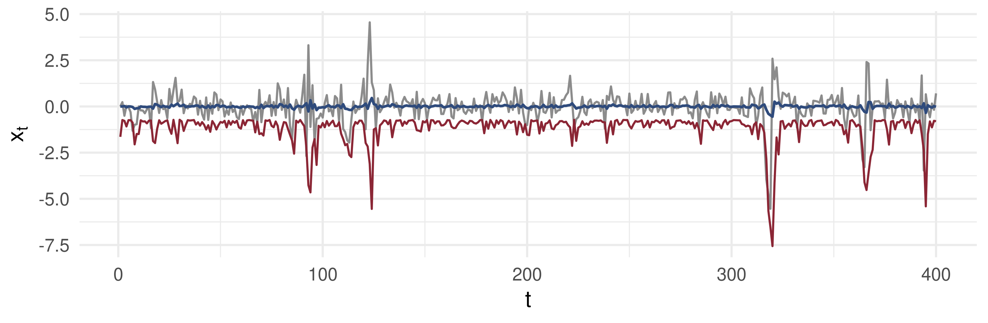
AR(1)-ARCH(1): the mean barely moves, the 5% quantile does
n <- 400; r <- e <- s2 <- numeric(n); s2[1] <- 1
for (t in 2:n) {
  s2[t] <- 0.2 + 0.7 * e[t - 1]^2            # conditional variance
  e[t]  <- sqrt(s2[t]) * rnorm(1)
  r[t]  <- 0.1 * r[t - 1] + e[t]             # conditional mean 0.1 r_{t-1}
}
d <- data.frame(t = 1:n, r = r, mu = c(0, 0.1 * r[-n]), s = sqrt(s2))
ggplot(d, aes(t)) + geom_line(aes(y = r), colour = "grey55") +
  geom_line(aes(y = mu), colour = "#2f4b7c", linewidth = 1) +
  geom_line(aes(y = mu - 1.645 * s), colour = "#8b2635", linewidth = 0.8) +
  labs(x = "t", y = expression(x[t]))

Blue: \(\mu_t\). Red: the conditional 5% quantile \(\mu_t - 1.645\,\sigma_t\). A mean model would call this series nearly unpredictable; a quantile model would not.

🧭 Model Selection: the Principle

Selection runs object → class of models → specific model.

Object Class Specific models
\(\mu_t\) AR AR(1), AR(2), …
\(\mu_t\) TAR (threshold AR) TAR(1,1,1), …
\(\mu_t\) MSW (Markov switching) two-regime AR, …

Workflow: (1) specify the object, (2) collect the data, (3) choose the model, (4) select within and across classes. Step 4 is the hard one. The model is an approximation to the data-generating process (DGP), not the DGP itself.

🔧 Tool 1: Diagnostic Testing

Does the estimated model conform to its own assumptions? Test, on the residuals:

  • no serial correlation (Ljung–Box, Breusch–Godfrey);
  • no conditional heteroskedasticity;
  • normality, if it was assumed (Jarque–Bera);
  • parameter stability (Andrews’ sup-type test);
  • a correct distributional assumption: the probability integral transforms \(u_t = F_{t-1}(x_t)\) should be i.i.d. \(U(0,1)\).

A failed diagnostic says the model is wrong; a passed one does not say it is right.

🔧 Tool 2: Sequential Testing

Shape the model by testing parameter restrictions.

(A) General-to-specific (GETS). Start from a large \(AR(\bar p)\) and test \(H_0: \phi_{\bar p} = 0\).

  • \(H_0\) rejected → keep \(AR(\bar p)\) and stop.
  • \(H_0\) not rejected → move to \(AR(\bar p - 1)\) and test \(\phi_{\bar p - 1} = 0\).

Only restrictions the data accept are imposed.

(B) Specific-to-general. Start small and relax restrictions that are rejected. It fails, in general: every test is run inside a model that is still misspecified, so its size and power are not what the tables say.

🔧 Tool 3: Information Criteria

Choose the model that minimises \[IC(k) = \underbrace{-2\log\hat{\mathcal L}_k}_{\text{quality of fit}} + \underbrace{f(k)}_{\text{complexity}},\] with \(k\) the number of parameters and \(f\) increasing.

Criterion Penalty \(f(k)\)
Akaike (AIC) \(2k\)
Schwarz / Bayesian (SIC, BIC) \(k \log T\)
Hannan–Quinn (HQ) \(2k \log\log T\)

For \(T \ge 8\), \(\log T > 2\): BIC punishes each parameter harder than AIC, and HQ lies between them for \(T > 16\).

✏️ Information Criteria for an AR(p)

With Gaussian errors, the maximised log-likelihood of an AR(\(p\)) on \(T\) observations is \[\log\hat{\mathcal L} = -\tfrac T2\log(2\pi) - \tfrac T2\log\hat\sigma_p^2 - \tfrac T2, \qquad \hat\sigma_p^2 = \tfrac1T\textstyle\sum_t \hat\varepsilon_t^2.\]

Dropping the constants, every criterion becomes \[IC(p) = T\log\hat\sigma_p^2 + f(p+1),\] where \(k = p+1\) counts the slopes and the intercept. Dividing by \(T\) gives the per-observation form \(\log\hat\sigma^2_p + 2k/T\) for AIC.

Adding a lag never raises \(\hat\sigma_p^2\). The penalty is the only thing that stops the search at a finite \(p\). Compare all orders on the same sample: lose the first \(\bar p\) observations for every \(p\).

🧮 Worked Example: Pick an Order

\(T = 100\) observations; residual variances from AR(\(p\)), \(p = 0, \dots, 3\). Penalty per parameter: AIC \(2\), BIC \(\log 100 = 4.61\).

\(p\) \(\hat\sigma_p^2\) \(100\log\hat\sigma_p^2\) AIC BIC
0 1.500 40.55 42.55 45.15
1 1.200 18.23 22.23 27.44
2 1.150 13.98 19.98 27.79
3 1.130 12.22 20.22 30.64

AIC chooses \(p = 2\) (19.98). BIC chooses \(p = 1\) (27.44 < 27.79): the second lag lowers \(T\log\hat\sigma^2\) by 4.25, more than AIC’s price of 2 but less than BIC’s 4.61.

✏️ Why AIC Overfits

Let the true order be \(p_0\), and let it be in the candidate set. Compare \(p_0\) with \(p_0 + 1\).

The gain in fit from the redundant lag is the likelihood-ratio statistic, \[T\log\big(\hat\sigma^2_{p_0}/\hat\sigma^2_{p_0+1}\big) \xrightarrow{d} \chi^2_1 .\] The criterion adds the lag when that gain exceeds the extra penalty \(c_T = f(k+1) - f(k)\):

  • AIC: \(c_T = 2\), so \(\Pr(\chi^2_1 > 2) = 0.157\) for every \(T\);
  • BIC: \(c_T = \log T \to \infty\), so the probability tends to \(0\).

✏️ Why BIC Is Consistent

Underfitting. Drop a true lag and \(\hat\sigma^2\) converges to a strictly larger number, so \(T\log\hat\sigma^2\) rises by an amount of order \(T\). Any penalty with \(c_T/T \to 0\) is outweighed, and the short model loses.

Consistency

A criterion selects \(p_0\) with probability tending to one if its per-parameter penalty satisfies \(c_T \to \infty\) and \(c_T/T \to 0\), and the true model is among finitely many candidates.

BIC (\(\log T\)) and HQ (\(2\log\log T\)) satisfy both; HQ’s is the slowest-growing penalty that still does. AIC fails the first.

💻 AIC vs BIC as \(T\) Grows

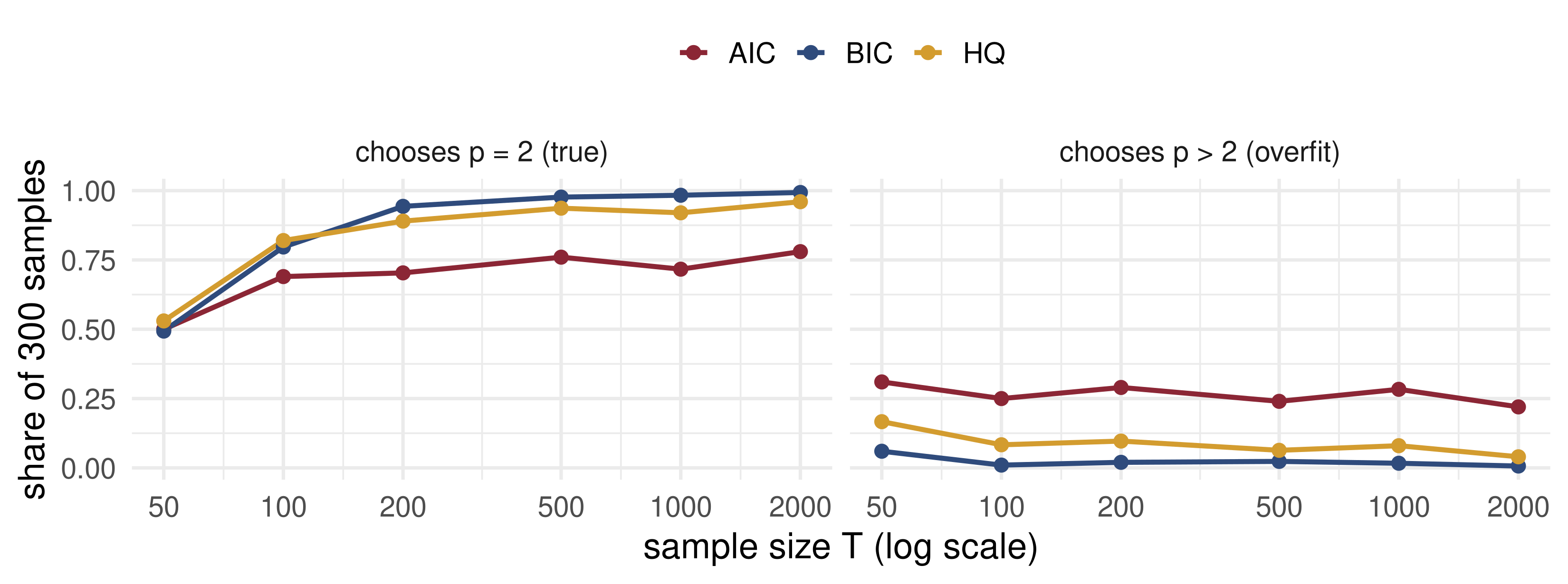
DGP: AR(2) with \(\phi = (0.5, -0.3)\); candidates \(p = 0, \dots, 8\). BIC’s hit rate climbs to 1; AIC’s overfit share stays near 0.27 for every \(T\).

🎛️ Explore: the IC Curves

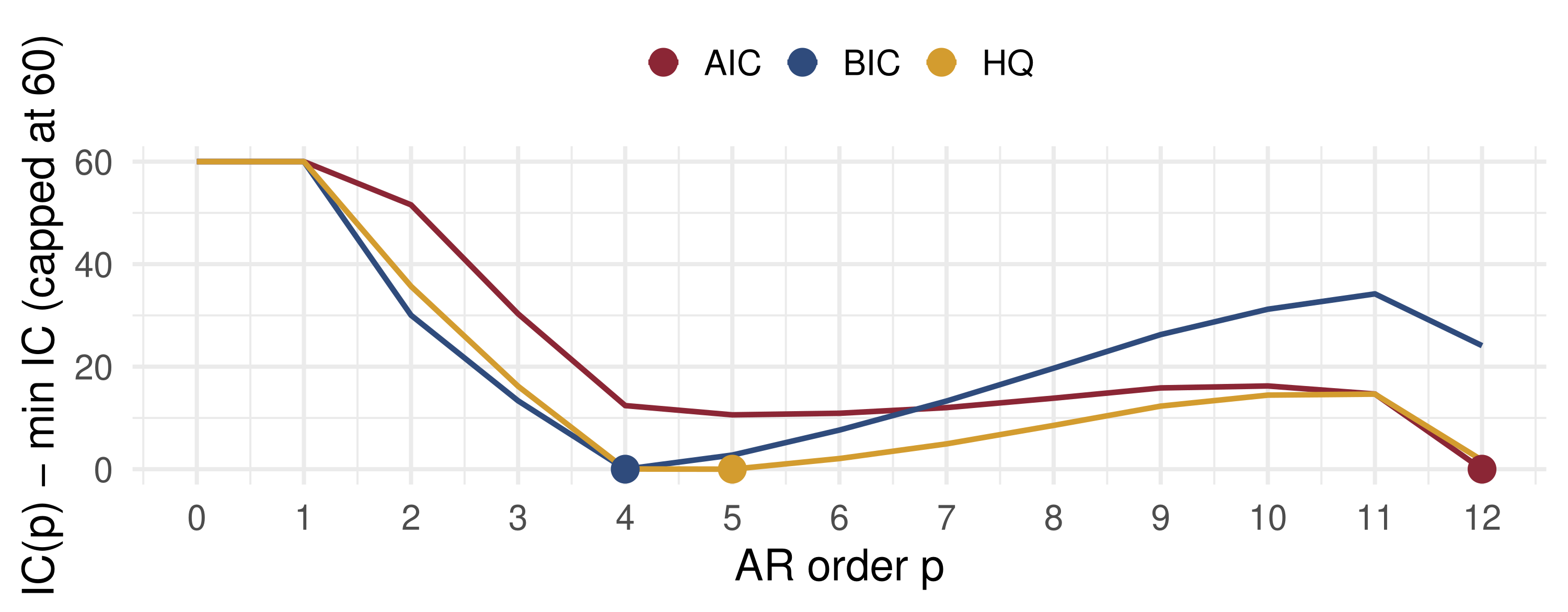
🎛️ What the Curves Show

The true order is \(p_0 = 2\). Large dots mark each criterion’s choice.

  • To the left of \(p_0\) all three curves are steep, and the steepness grows with \(T\): underfitting costs order \(T\).
  • To the right of \(p_0\) AIC’s curve is nearly flat. A lucky lag can tip it, at any \(T\).
  • BIC’s right-hand side climbs by about \(\log T\) per lag, so at \(T = 2000\) it rises by 7.6 per lag and noise cannot overturn that.
  • At \(T = 30\), try a few samples: BIC often stops at \(p = 1\). Consistency is a large-sample property.

🧠 Think-Pair-Share

An analyst fits AR(\(p\)), \(p = 0, \dots, 4\), to \(T = 200\) monthly observations and reports \(200\log\hat\sigma_p^2\):

\(p\) 0 1 2 3 4
\(200\log\hat\sigma^2_p\) 60.0 31.0 24.0 20.0 18.5
  1. Which order does AIC choose? Which does BIC (\(\log 200 = 5.30\))?
  2. Starting from \(\bar p = 4\), a GETS search finds \(|t| = 1.1\) for \(\hat\phi_4\) and \(|t| = 2.4\) for \(\hat\phi_3\). Where does it stop?

✅ Think-Pair-Share: Solution

  1. Add \(2(p+1)\) for AIC and \(5.30(p+1)\) for BIC:
\(p\) 0 1 2 3 4
AIC 62.0 35.0 30.0 28.0 28.5
BIC 65.3 41.6 39.9 41.2 45.0

AIC picks \(p = 3\); BIC picks \(p = 2\). The third lag gains 4.0 in fit: above 2, below 5.30.

  1. \(\phi_4 = 0\) is not rejected (\(1.1 < 1.96\)), so drop to AR(3). \(\phi_3 = 0\) is rejected (\(2.4 > 1.96\)), so GETS stops at AR(3), as AIC did. At the 5% level, GETS behaves like a criterion with a per-lag price of \(1.96^2 \approx 3.84\).

💰 Case Study: Unemployment Lags

📈 The question

How many lags of its own past does the monthly change in US unemployment need?

  1. Which orders do AIC, BIC and HQ choose?
  2. Where does GETS from \(\bar p = 12\) stop?
  3. Are the chosen model’s residuals white noise?

📊 The data

Series: civilian unemployment rate (FRED UNRATE), seasonally adjusted

Period: Jan 1960 – Dec 2019, 720 months (the 2020 pandemic jump left out)

\(x_t = U_t - U_{t-1}\), percentage points

u <- read.csv("https://fred.stlouisfed.org/graph/fredgraph.csv?id=UNRATE")

💰 Case Study: Three Criteria and GETS

📦 AR(0)–AR(12): criteria, GETS, Ljung–Box
u <- read.csv("data/UNRATE.csv"); x <- diff(u$UNRATE)
pmax <- 12; X <- embed(x, pmax + 1); y <- X[, 1]; n <- length(y)
fits <- lapply(0:pmax, function(p) if (p == 0) lm(y ~ 1) else lm(y ~ X[, 1 + seq_len(p)]))
s2 <- sapply(fits, function(f) mean(resid(f)^2)); k <- 1:(pmax + 1)
ic <- data.frame(p = 0:pmax, AIC = n*log(s2) + 2*k, BIC = n*log(s2) + k*log(n),
                 HQ = n*log(s2) + 2*k*log(log(n)))
p_ic <- sapply(ic[, -1], which.min) - 1
p <- pmax                                 # GETS: drop the last lag while |t| < 1.96
while (p > 0 && abs(coef(summary(fits[[p + 1]]))[p + 1, 3]) < 1.96) p <- p - 1
lb <- sapply(c(p_ic, GETS = p), function(q) Box.test(resid(fits[[q + 1]]), lag = 24,
                                                       type = "Ljung", fitdf = q)$p.value)
data.frame(rule = names(lb), order = c(p_ic, p), LjungBox24_pval = signif(lb, 2), row.names = NULL)
  rule order LjungBox24_pval
1  AIC    12         0.00036
2  BIC     4         0.00014
3   HQ     5         0.00027
4 GETS    12         0.00036

The criteria disagree by eight lags; every residual series fails the Ljung–Box test at lag 24.

💰 Case Study: What the Data Say

What the data say: BIC stops at 4 lags, HQ at 5; AIC and GETS run to the boundary at 12. Even AR(12) fails Ljung–Box: its residuals keep a correlation of −0.18 at lag 24, a trace of seasonal adjustment. And unemployment rises fast and falls slowly, an asymmetry no linear AR captures (Lecture 11).

📝 Quiz #1: The Right Object

A bank must hold capital against the loss it will exceed on only 1% of days. Which object of the daily return distribution should it model?

  • The conditional 1% quantile \(q_t^{0.01}\)
  • The conditional mean \(\mu_t\)
  • The conditional skewness \(S_t/\sigma_t^3\)
  • The unconditional variance of returns

📝 Quiz #2: Overfitting Rate

The true model is AR(1) and the candidates are AR(1) and AR(2) only. As \(T \to \infty\), how often does AIC choose AR(2)?

  • About 15.7% of the time, for every large \(T\)
  • With probability tending to zero
  • About 5% of the time
  • Never, because the second coefficient is zero

📝 Quiz #3: GETS

In a general-to-specific search, the test of \(H_0: \phi_{\bar p} = 0\) in \(AR(\bar p)\) is not rejected. What is the next step?

  • Move to \(AR(\bar p - 1)\) and test its last coefficient
  • Keep \(AR(\bar p)\) and stop
  • Move to \(AR(\bar p + 1)\)
  • Switch to an information criterion

📋 Key Formulas

Conditional mean \(\mu_t = E_{t-1}[x_t]\), minimises \(E[(x_t - g)^2]\) over \(g \in I_{t-1}\)
Conditional variance \(\sigma_t^2 = E_{t-1}[(x_t - \mu_t)^2]\)
Conditional quantile \(\Pr_{t-1}\{x_t \le q_t^\alpha\} = \alpha\); median at \(\alpha = 0.5\)
Information criterion \(IC(k) = -2\log\hat{\mathcal L}_k + f(k)\) → min
AR(\(p\)), Gaussian \(IC(p) = T\log\hat\sigma_p^2 + f(p+1)\)
Penalties AIC \(2k\); BIC \(k\log T\); HQ \(2k\log\log T\)
Consistency penalty per parameter \(c_T \to \infty\), \(c_T/T \to 0\)

📋 Summary

  • Non-structural modelling begins by choosing an object: a feature of the distribution of \(x_t\) given its past.
  • The conditional mean is optimal under squared loss, the median under absolute loss, a quantile under check loss.
  • Selection runs object → class → model; diagnostics, GETS and information criteria are the tools.
  • BIC and HQ are consistent; AIC overfits with positive probability at every \(T\), which is not always a defect when the goal is prediction.
  • All of these criteria judge in-sample fit.

📚 Further Reading and Next Lecture

  • Hamilton (1994), Time Series Analysis, ch. 4–5.
  • Tsay (2010), Analysis of Financial Time Series, ch. 2.4–2.5 (order selection).
  • Franses and van Dijk (2000), Non-Linear Time Series Models in Empirical Finance, ch. 2.
  • Akaike (1974); Schwarz (1978); Hannan and Quinn (1979), the three criteria.
  • Hendry (1995), Dynamic Econometrics, on general-to-specific modelling.

Next lecture: In-Sample Fit, Out-of-Sample Forecasts, Diebold–Mariano. A model that fits well in sample often forecasts badly. Why, and how do we test it?