Time Series Econometrics

Lecture 5: In-Sample Fit, Out-of-Sample Forecasts, Diebold–Mariano

Samir Orujov, PhD

Open lecture notes, after Stanislav Anatolyev’s course (2016)

🎬 The Idea in 3 Minutes

⬅ Previous lecture: 4 · What to Model, and How to Choose a Model

A short film with the intuition. Watch it before the slides, or after. Captions: CC button.

🎯 Learning Objectives

By the end of this lecture, you will be able to:

• Explain why a model that fits well in sample can forecast badly
• Derive the forecast cost of one redundant parameter, \(\sigma^2(1 + 1/T)\)
• Construct out-of-sample forecasts under fixed, rolling and recursive schemes
• Compute the Diebold–Mariano statistic with a HAC long-run variance
• State when the DM test is not valid: nested models and parameter uncertainty

🔁 Warm-up from last time

The true model is an AR(2) and the candidates are AR(0) to AR(8). As \(T \to \infty\), which statement is true?

• BIC chooses AR(2) with probability tending to one; AIC overfits with positive probability
• AIC and BIC both choose AR(2) with probability tending to one
• AIC chooses AR(2) with probability tending to one; BIC underfits
• Both overfit with positive probability, since adding a lag never raises \(\hat\sigma^2\)

🗺️ Where We Are

Lecture 4 chose models with diagnostic tests, GETS and information criteria. Every one of these tools looks at the same data the model was estimated on: they measure in-sample fit.

But the second aim of non-structural modelling was prediction: \(\hat x_{T+1|T}\), a value we have not yet seen. Today we judge models by what they do on data they were not fitted to, and we build a test that says whether one forecast is really better than another.

❓ The Question

Can a model beat “no change”?

To forecast next month’s inflation, the simplest rule is the random walk: next month equals this month. An autoregression uses more of the past and fits the history better.

Does it forecast better? Atkeson and Ohanian (2001) found that elaborate inflation models often did not beat a naive rule out of sample. A lower forecast error in one sample can be luck. We need a test.

📐 In-Sample vs Out-of-Sample Fit

• In-sample fit: the ability to explain the data.
• Out-of-sample fit: the ability to forecast.

Often a model that fits well in sample performs badly out of sample. Three reasons:

1. Structural breaks: the DGP changes, unpredictably, after the estimation period.
2. Over-parameterisation: a model that fits well usually has more parameters, and each estimated parameter adds noise to the forecast.
3. Data mining: searching a large set of models selects one that fits the sample’s accidents, not the DGP.

✏️ The Cost of One Redundant Parameter

Let the true model be strong white noise, \(x_t = \varepsilon_t\), \(\operatorname{Var}\varepsilon_t = \sigma^2\). The optimal forecast is \(x_{T+1|T} = 0\), with MSPE \(\sigma^2\).

Estimate instead \(x_t = c + \varepsilon_t\). Then \(\hat c = \bar x_T\) and \(\hat x_{T+1|T} = \hat c\). Since \(\varepsilon_{T+1}\) is independent of \(\hat c\), \[E\big[(x_{T+1} - \hat c)^2\big] = E[\varepsilon_{T+1}^2] + E[\hat c^2] = \sigma^2 + \frac{\sigma^2}{T} = \sigma^2\Big(1 + \frac1T\Big).\]

The redundant parameter fits the sample better (it absorbs \(\bar x_T\)) and forecasts worse. With \(k\) estimated parameters the same algebra gives approximately \(\sigma^2(1 + k/T)\): the price is small per parameter, and it grows with every one.

💻 Predicting White Noise

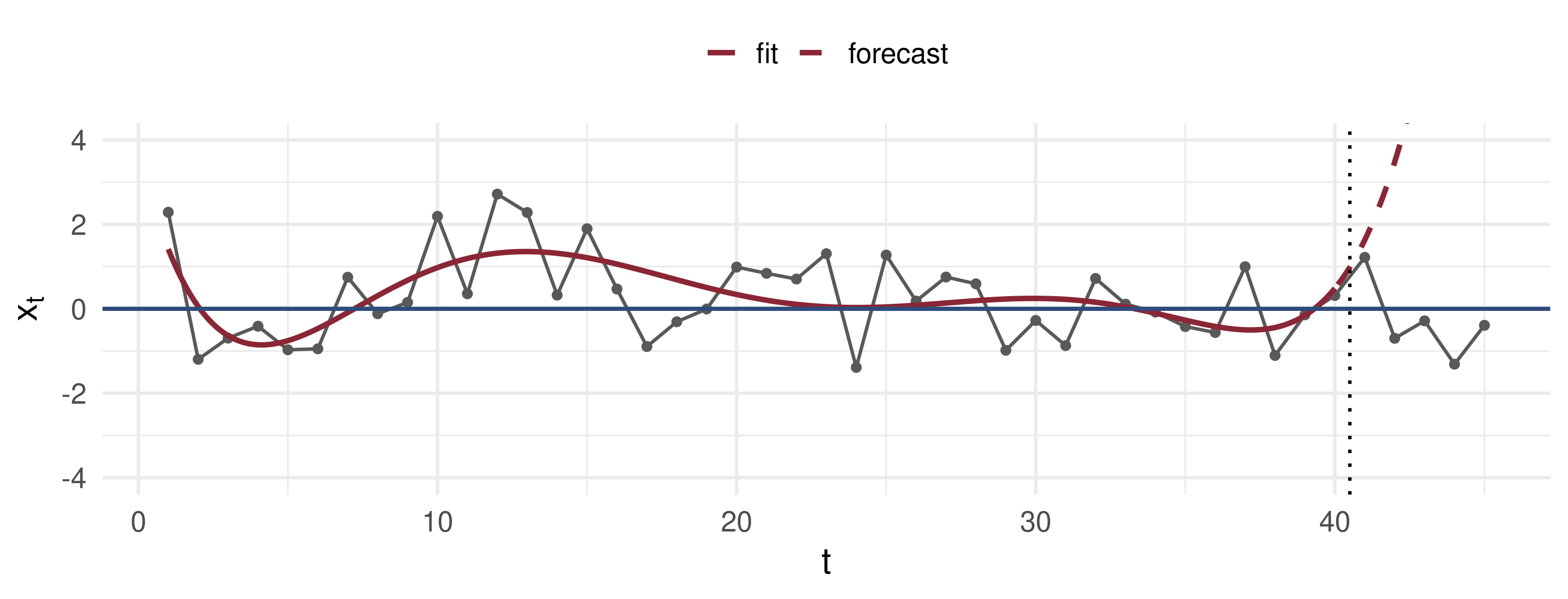
Grey: white noise, \(x_t = \varepsilon_t\). Red: a degree-6 polynomial in \(t\), fitted to \(t \le 40\) and extrapolated. Blue: the optimal forecast, 0.

💻 Fit Falls, Forecast Error Explodes

one <- function() {
  x <- rnorm(45); Z <- function(t, d) outer(t / 40, 0:d, "^")
  sapply(0:8, function(d) { b <- qr.solve(Z(1:40, d), x[1:40])
    c(in_sample_MSE  = mean((x[1:40]  - Z(1:40, d)  %*% b)^2),
      out_sample_MSPE = mean((x[41:45] - Z(41:45, d) %*% b)^2)) })
}
r <- apply(replicate(1000, one()), 1:2, mean)
colnames(r) <- paste0("d=", 0:8); round(r, 2)

                 d=0  d=1  d=2  d=3  d=4   d=5   d=6    d=7    d=8
in_sample_MSE   0.98 0.95 0.93 0.90 0.88  0.85  0.83   0.81   0.78
out_sample_MSPE 1.05 1.15 1.42 2.08 4.35 11.92 33.63 108.35 418.92

Average over 1,000 samples of 45 points (fit on 40, forecast 5), \(\sigma^2 = 1\). Each extra degree lowers the in-sample error a little and raises the forecast error a lot.

📐 Data Mining

Fit 100 models to one sample and keep the best. The winner is the model that best matched this sample’s idiosyncrasies, and part of its good fit is luck that will not repeat.

• Its in-sample fit is biased upwards.
• Its out-of-sample performance regresses towards the truth.
• A test that ignores the search treats the winner as if it had been chosen in advance.

The remedy is to judge models on data they have not seen, and, when many models are compared, to account for the search itself. The second half of that sentence is Lecture 6.

📐 Splitting the Sample

Split the \(T\) observations as \(T = R + P\):

\[\underbrace{1, \dots, R}_{\text{in sample: estimate}} \;\Big|\; \underbrace{R+1, \dots, R+P}_{\text{out of sample: forecast}}\]

1. Run the in-sample procedure (model selection, estimation) on the first part.
2. Construct the one-step forecasts \(\hat x_{R+p|R+p-1}\), \(p = 1, \dots, P\).
3. Compare \(P\) forecasts with \(P\) realisations: \[MSPE = \frac1P\sum_{p=1}^{P}\big(x_{R+p} - \hat x_{R+p|R+p-1}\big)^2 .\]

📐 Fixed, Rolling, Recursive

Which observations estimate the parameters used to forecast \(x_{R+p}\)?

Scheme	Estimation sample	Strength
Fixed	\(1, \dots, R\), once	cheap
Rolling	\(p, \dots, R+p-1\), the last \(R\)	robust to structural breaks
Recursive	\(1, \dots, R+p-1\), expanding	most observations; efficient if stable

The trade-off is bias against variance. A rolling window forgets old regimes but always estimates from \(R\) points; a recursive window keeps shrinking its estimation noise but averages across any break.

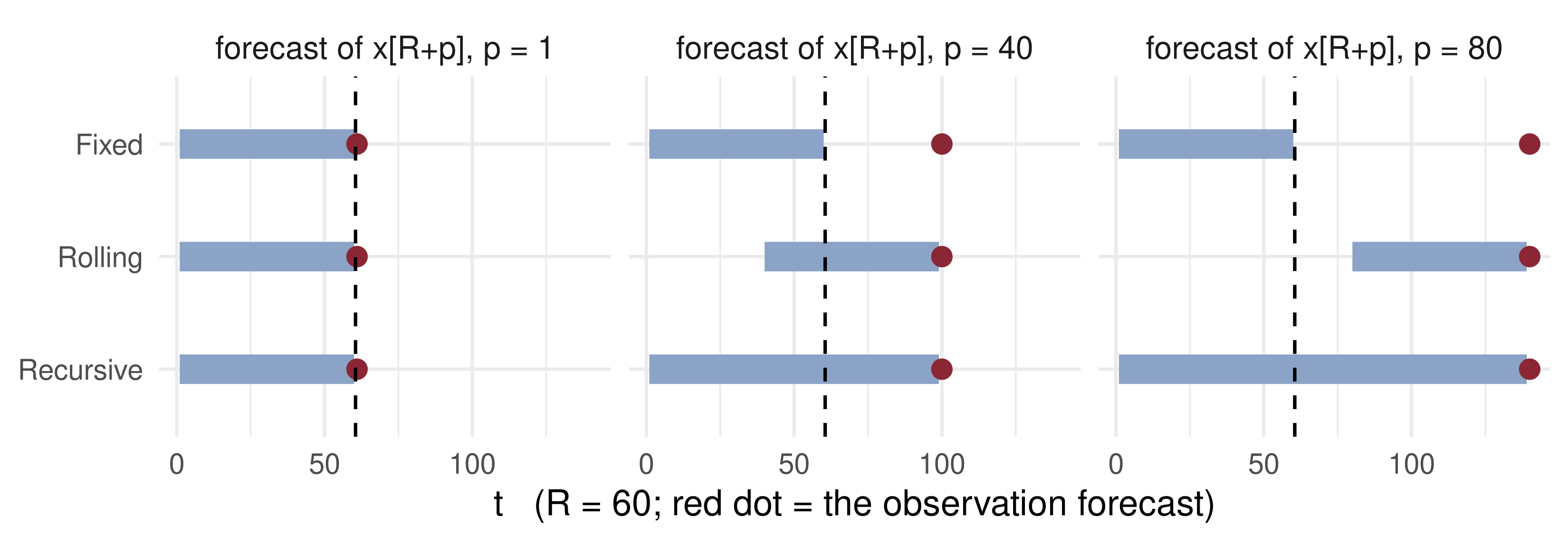
💻 The Three Windows

The bars are the estimation samples. Only the rolling bar keeps its length; only the fixed bar never moves.

🎛️ Explore: a Break

viewof delta = Inputs.range([0, 3], {step: 0.1, value: 0, label: "Mean shift δ at t = 150"})

brk = {
  let s = 12345;
  const u = () => { s = (s * 16807) % 2147483647; return s / 2147483647; };
  const z = () => Math.sqrt(-2 * Math.log(u())) * Math.cos(2 * Math.PI * u());
  const N = 300, R = 60, x = d3.range(N).map(t => (t >= 150 ? delta : 0) + z());
  const out = []; let cum = 0;
  for (let t = R; t < N; t++) {
    const rec = d3.mean(x.slice(0, t)), rol = d3.mean(x.slice(t - R, t));
    cum += (x[t] - rec) ** 2 - (x[t] - rol) ** 2;
    out.push({t, x: x[t], rec, rol, cum});
  }
  return out;
}

Plot.plot({
  width: 1100, height: 190, marginTop: 30, marginLeft: 78, marginRight: 110, style: {fontSize: "18px"},
  x: {label: null}, y: {label: "x and forecasts", domain: [-3, 6]},
  marks: [
    Plot.dot(brk, {x: "t", y: "x", r: 2, fill: "#aaaaaa"}),
    Plot.line(brk, {x: "t", y: "rec", stroke: "#2f4b7c", strokeWidth: 3}),
    Plot.line(brk, {x: "t", y: "rol", stroke: "#8b2635", strokeWidth: 3}),
    Plot.text([{t: 300, y: brk.at(-1).rec}], {x: "t", y: "y", text: () => "recursive", dx: 50, dy: 14, fontSize: 18, fill: "#2f4b7c"}),
    Plot.text([{t: 300, y: brk.at(-1).rol}], {x: "t", y: "y", text: () => "rolling", dx: 50, dy: -14, fontSize: 18, fill: "#8b2635"})
  ]
})

Plot.plot({
  width: 1100, height: 170, marginTop: 30, marginLeft: 78, marginRight: 110, marginBottom: 45, style: {fontSize: "18px"},
  x: {label: "t"}, y: {label: "Σ (e²rec − e²roll)"},
  marks: [Plot.ruleY([0]), Plot.ruleX([150], {strokeDasharray: "4,4"}),
          Plot.line(brk, {x: "t", y: "cum", stroke: "#d39c2f", strokeWidth: 3})]
})

🎛️ What the Explorable Shows

The series is \(x_t = \delta\,\mathbf 1\{t \ge 150\} + \varepsilon_t\); both schemes forecast with a sample mean, \(R = 60\). The lower panel cumulates the loss differential: rising means the rolling forecast is winning.

• \(\delta = 0\): the line drifts down. With no break, the recursive mean averages more data and has less estimation noise.
• \(\delta = 1.5\): after \(t = 150\) the line climbs. The recursive mean still remembers the old regime and adjusts slowly; the rolling mean catches up within 60 periods.
• Neither scheme wins everywhere. Which is better depends on how unstable the DGP is.

📐 Testing Equal Predictive Ability

Model A’s MSPE is smaller than model B’s. Is the difference significant, or chance?

Diebold and Mariano (1995). With forecast errors \(e_t^A\), \(e_t^B\), define the loss differential \[d_t = (e_t^A)^2 - (e_t^B)^2 .\]

\[H_0: E[d_t] = 0, \qquad H_A: E[d_t] < 0 \ \text{(A better)}, \qquad H_B: E[d_t] > 0 \ \text{(B better)}.\]

Any loss can replace the square: absolute error, an asymmetric loss, a trading profit.

📐 The DM Statistic

\[\bar d = \frac1P\sum_{p=1}^{P} d_{R+p}, \qquad DM = \frac{\sqrt P\,\bar d}{\sqrt{\hat\Omega}} \xrightarrow[H_0]{d} N(0,1),\] where \(\hat\Omega\) estimates the long-run variance of \(d_t\), \(\Omega = \sum_{j=-\infty}^{\infty}\operatorname{Cov}(d_t, d_{t-j})\).

This is Lecture 2’s CLT applied to the stationary, ergodic series \(d_t\): \(\sqrt P(\bar d - E d_t) \xrightarrow{d} N(0, \Omega)\). Use a HAC estimator, e.g. Newey–West, for \(\Omega\).

Two-sided test: reject when \(|DM| > 1.96\) at 5%. Under \(H_A\), \(DM \to -\infty\) (left tail, A better); under \(H_B\), \(DM \to +\infty\) (right tail, B better).

✏️ Why a HAC Variance?

Take an AR(1), \(x_t = \rho x_{t-1} + \varepsilon_t\). The optimal \(h\)-step forecast is \(\rho^h x_t\), and its error is \[x_{t+h} - \rho^h x_t = \varepsilon_{t+h} + \rho\,\varepsilon_{t+h-1} + \dots + \rho^{h-1}\varepsilon_{t+1}.\]

For \(h = 2\) the errors of the forecasts made at \(t\) and \(t+1\) both contain \(\varepsilon_{t+2}\). So \(h\)-step errors are MA(\(h-1\)), and \(d_t\) inherits autocorrelation up to lag \(h - 1\).

One-step errors of an optimal forecast are not autocorrelated, but forecasts from misspecified or estimated models need not be optimal. A HAC estimator costs little when it is not needed and protects when it is.

🧮 Worked Example: A DM Test by Hand

\(P = 100\) one-step forecasts. \(\bar d = -0.6\); sample autocovariances of \(d_t\): \(\hat\gamma_0 = 4.0\), \(\hat\gamma_1 = 1.2\), higher ones negligible.

Newey–West with \(m = 1\). \(\hat\Omega = \hat\gamma_0 + 2\big(1 - \tfrac12\big)\hat\gamma_1 = 4.0 + 1.2 = 5.2\). \[DM = \frac{\sqrt{100}\times(-0.6)}{\sqrt{5.2}} = \frac{-6}{2.280} = -2.63 .\]

\(|DM| > 1.96\) and \(DM < 0\): reject \(H_0\) in favour of \(H_A\), A forecasts better. Ignoring the autocorrelation (\(\hat\Omega = \hat\gamma_0 = 4\)) would give \(-3.0\): the right answer here, with a statistic overstated by 14%.

⚠️ Caveat 1: Nested Models

DM is for non-nested models.

If B is A plus extra parameters, then under \(H_0\) the extra parameters are zero and both models have identical population errors. The loss differential \(d_t\) degenerates to zero, its long-run variance is zero, and the \(N(0,1)\) limit fails.

In finite samples the larger model’s estimation noise makes \(\bar d\) systematically signed, against the larger model. Use the Clark–McCracken or Clark–West tests instead.

With a rolling window of fixed length, Giacomini and White (2006) show that the DM statistic tests the forecasting methods, estimation noise included, and stays valid for nested models. Not in the 2016 notes.

⚠️ Caveat 2: Parameter Uncertainty

The forecasts are built from estimated parameters, so the errors \(\hat e_t\) carry estimation error as well as the innovation.

West (1996): the asymptotic variance of \(\sqrt P\,\bar d\) in general needs a correction for this. The result is the Diebold–Mariano–West framework.

The correction vanishes asymptotically in important special cases:

• MSPE loss with models estimated by OLS;
• \(P/R \to 0\): the evaluation sample is small relative to the estimation sample.

🧠 Think-Pair-Share

Two forecasters predict monthly Brent oil price changes. Over \(P = 144\) months, \(d_t = (e_t^A)^2 - (e_t^B)^2\) has mean \(\bar d = 0.15\), and a Newey–West estimate of its long-run variance is \(\hat\Omega = 2.25\).

1. Compute \(DM\). Which forecaster had the smaller MSPE in this sample? Is the difference significant at 5%?
2. Model B is model A plus three extra lags. Should you trust the \(N(0,1)\) critical value?
3. Brent’s mean return shifted in 2014. Which estimation scheme would you prefer, and why?

✅ Think-Pair-Share: Solution

1. \(DM = \sqrt{144}\times 0.15/\sqrt{2.25} = 12 \times 0.15/1.5 = 1.2\). \(\bar d > 0\), so B had the smaller MSPE, but \(1.2 < 1.96\): the difference is not significant. The sample cannot tell the forecasters apart.

2. No. The models are nested, so under \(H_0\) the loss differential degenerates and DM is not \(N(0,1)\); the larger model’s estimation noise biases \(\bar d\) against it. Use Clark–West, or a fixed-length rolling window and the Giacomini–White argument.

3. Rolling. After a break, a recursive window keeps averaging over the old regime; a rolling window discards it after \(R\) months.

💰 Case Study: AR vs Random Walk

📈 The question

Does an AR(3) forecast next month’s US inflation better than the random walk \(\hat\pi_{t+1} = \pi_t\)?

1. What are the out-of-sample MSPEs under the fixed, rolling and recursive schemes?
2. Is the AR’s advantage significant by DM?
3. When did the AR gain its advantage?

📊 The data

Series: CPI, all urban consumers, SA (FRED CPIAUCSL)

Period: Jan 1990 – Sep 2025, 429 months; \(R = 120\) (1990s), \(P = 309\)

\(\pi_t = 1200\,\Delta\log CPI_t\), annualised % per month

cpi <- read.csv("https://fred.stlouisfed.org/graph/fredgraph.csv?id=CPIAUCSL")

💰 Case Study: MSPE and DM in R

library(sandwich)
c0 <- read.csv("data/CPIAUCSL.csv"); dates <- as.Date(c0$observation_date[-1])
pi <- 1200 * diff(log(c0$CPIAUCSL)); N <- length(pi); R <- 120; P <- N - R; p <- 3
ar_fc <- function(scheme) sapply(1:P, function(j) {
  idx <- switch(scheme, fixed = 1:R, rolling = j:(R + j - 1), recursive = 1:(R + j - 1))
  X <- embed(pi[idx], p + 1); b <- lm.fit(cbind(1, X[, -1]), X[, 1])$coefficients
  sum(b * c(1, pi[(R + j - 1):(R + j - p)]))            # forecast of pi[R + j]
})
y <- pi[(R + 1):N]; e_rw <- y - pi[R:(N - 1)]
dm <- function(e_a, e_b) { d <- e_a^2 - e_b^2
  m <- floor(4 * (P / 100)^(2 / 9))                       # Newey-West lag, = 5 here
  mean(d) / sqrt(NeweyWest(lm(d ~ 1), lag = m, prewhite = FALSE)[1, 1]) }
e_ar <- sapply(c("fixed", "rolling", "recursive"), function(s) y - ar_fc(s))
rbind(MSPE_AR = colMeans(e_ar^2), MSPE_RW = mean(e_rw^2),
      DM_AR_vs_RW = apply(e_ar, 2, dm, e_b = e_rw)) |> round(2)

            fixed rolling recursive
MSPE_AR     11.13   10.66     10.29
MSPE_RW     13.68   13.68     13.68
DM_AR_vs_RW -2.18   -2.44     -2.91

Negative DM means the AR (model A) forecasts better; compare each with \(-1.96\).

💰 Case Study: What the Data Say

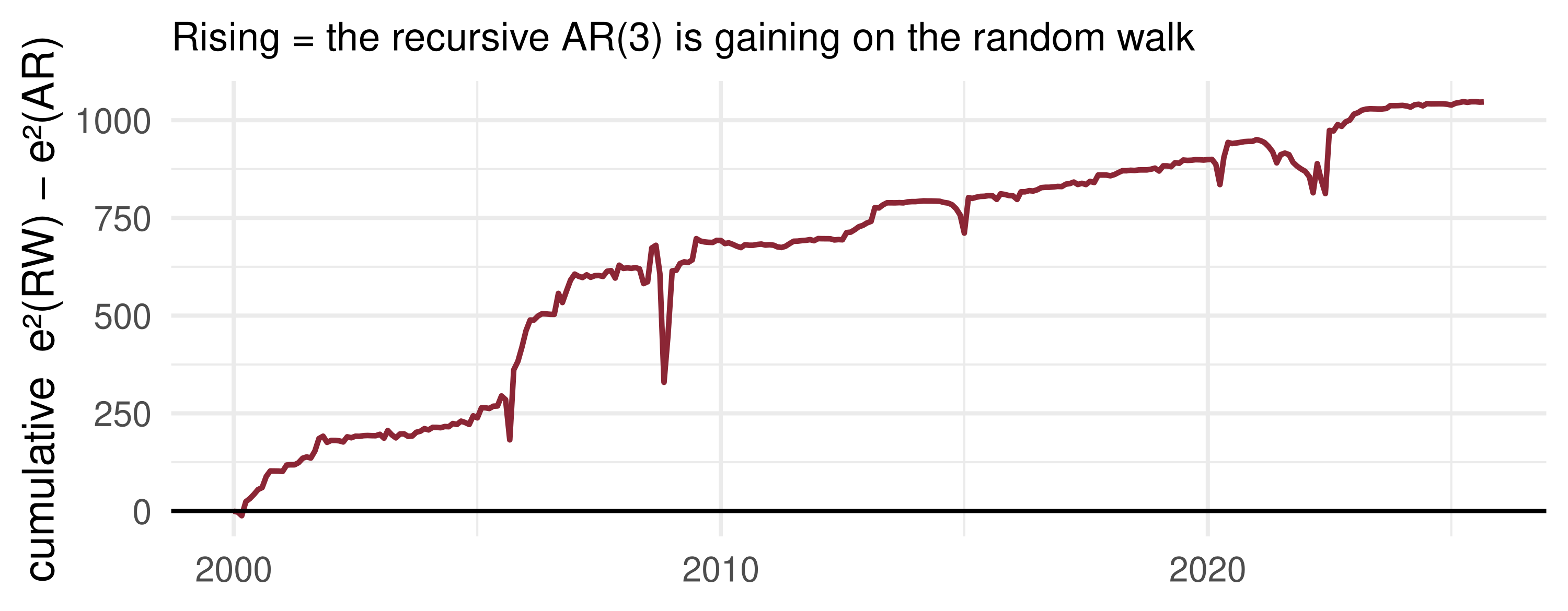
What the data say: the AR(3) beats the random walk under every scheme, significantly at 5%, and the recursive scheme does best. The gains arrive in jumps (2005–06, 2008–09, 2022–23), when inflation swung hard and “no change” was badly wrong; the downward spikes are the AR’s own bad months. In quiet years the two are nearly tied.

📝 Quiz #1: A Redundant Constant

The DGP is \(x_t = \varepsilon_t\) with \(\operatorname{Var}\varepsilon_t = 4\). You forecast with the sample mean of \(T = 50\) observations. What is the MSPE?

• \(4.08\)
• \(4.00\)
• \(4.80\)
• \(0.08\)

📝 Quiz #2: The Rolling Window

With in-sample size \(R\), which observations does the rolling scheme use to forecast \(x_{R+p}\)?

• \(x_p, \dots, x_{R+p-1}\)
• \(x_1, \dots, x_{R+p-1}\)
• \(x_1, \dots, x_R\)
• \(x_{p-1}, \dots, x_{R+p-1}\)

📝 Quiz #3: DM Variance

Why does the Diebold–Mariano statistic use a HAC estimate of the variance of \(d_t\)?

• Because \(d_t\) may be serially correlated, e.g. multi-step errors are MA(\(h-1\))
• Because \(d_t\) is not stationary under \(H_0\)
• Because the forecast errors are not normally distributed
• Because the models are nested

📋 Key Formulas

Redundant constant	\(E(x_{T+1} - \hat c)^2 = \sigma^2(1 + 1/T)\)
Out-of-sample MSPE	\(\frac1P\sum_{p=1}^P (x_{R+p} - \hat x_{R+p|R+p-1})^2\)
Fixed / rolling / recursive	estimate on \(1..R\) / \(p..R{+}p{-}1\) / \(1..R{+}p{-}1\)
Loss differential	\(d_t = (e_t^A)^2 - (e_t^B)^2\)
Diebold–Mariano	\(DM = \sqrt P\,\bar d/\sqrt{\hat\Omega} \xrightarrow{d} N(0,1)\) under \(H_0: E d_t = 0\)
Newey–West	\(\hat\Omega = \hat\gamma_0 + 2\sum_{j=1}^{m}\big(1 - \frac{j}{m+1}\big)\hat\gamma_j\)

📋 Summary

• In-sample fit and forecasting ability are different things; breaks, extra parameters and data mining drive them apart.
• Each redundant parameter costs about \(\sigma^2/T\) of forecast MSE.
• Evaluate on held-out data: split \(T = R + P\); choose a fixed, rolling or recursive scheme by how stable you believe the DGP to be.
• Diebold–Mariano tests \(E d_t = 0\) with a HAC long-run variance; it needs non-nested models, and West (1996) on parameter uncertainty.
• With many models, the best DM statistic is itself the product of a search.

📚 Further Reading and Next Lecture

• Diebold and Mariano (1995), “Comparing predictive accuracy”, JBES.
• West (1996), “Asymptotic inference about predictive ability”, Econometrica.
• Clark and West (2007), on nested models; Giacomini and White (2006), on conditional predictive ability.
• Atkeson and Ohanian (2001), “Are Phillips curves useful for forecasting inflation?”
• Hamilton (1994), ch. 4; Tsay (2010), ch. 2.

Next lecture: Data Snooping, Superior Predictive Ability, Model Confidence Sets. Test one hundred trading rules and the best looks brilliant. How do we test it honestly?