Time Series Econometrics

Lecture 6: Data Snooping, Superior Predictive Ability, Model Confidence Sets

Samir Orujov, PhD

Open lecture notes, after Stanislav Anatolyev’s course (2016)

🎬 The Idea in 3 Minutes

⬅ Previous lecture: 5 · In-Sample Fit, Out-of-Sample Forecasts, Diebold–Mariano

A short film with the intuition. Watch it before the slides, or after. Captions: CC button.

🎯 Learning Objectives

By the end of this lecture, you will be able to:

  • Explain why the best of many models looks significant even when none is
  • State the null hypothesis of superior predictive ability against a benchmark
  • Compute White’s Reality Check \(p\)-value with a block bootstrap
  • Describe how Hansen’s SPA test corrects the Reality Check for poor models
  • Construct a model confidence set by sequential elimination

🔁 Warm-up from last time

Over \(P = 100\) forecasts, the loss differential \(d_t = (e_t^A)^2 - (e_t^B)^2\) has \(\bar d = 0.3\) and HAC long-run variance \(\hat\Omega = 4\). What does the Diebold–Mariano test conclude at 5%?

  • \(DM = 1.5\): no significant difference between A and B
  • \(DM = 1.5\): B is significantly better
  • \(DM = 7.5\): A is significantly better
  • \(DM = 0.15\): A is significantly better

🗺️ Where We Are

Lecture 5 compared two forecasts with the Diebold–Mariano test, and ended on a warning: with many models, the best DM statistic is itself the product of a search.

Today we take the search seriously. First: does any of \(m\) models beat a benchmark? Then: which models could be the best one?

❓ The Question

One hundred trading rules

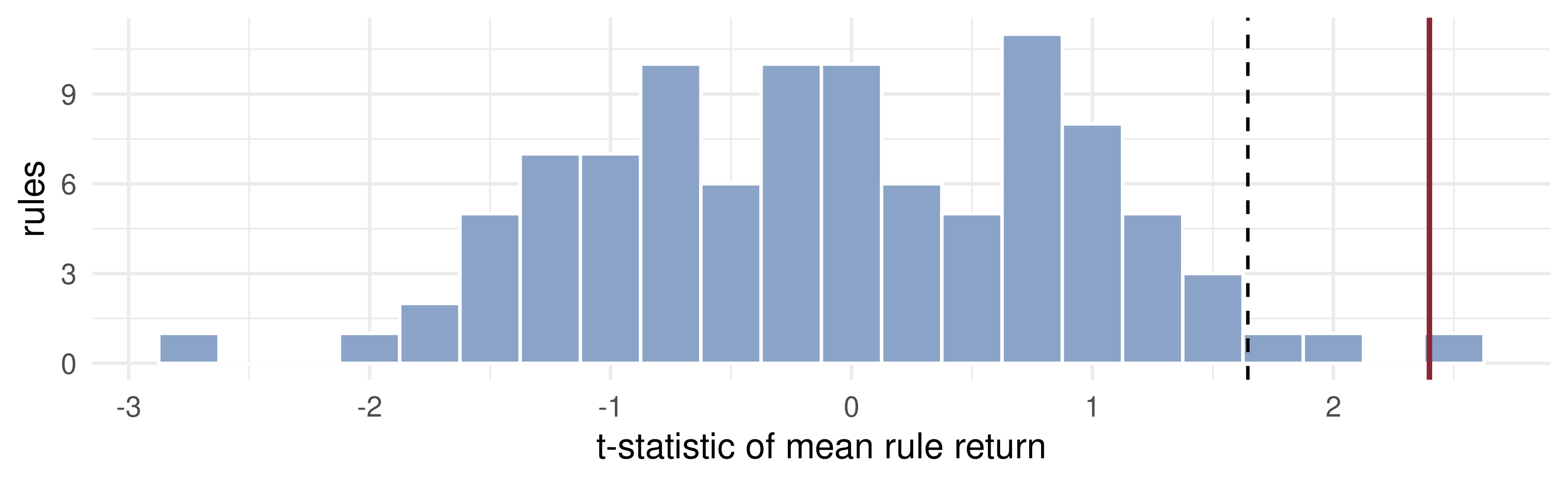
An analyst back-tests 100 trading rules on 500 days of returns. The best one earns a \(t\)-statistic of 2.4 against holding cash: a one-sided \(p\)-value of 0.008.

Does the fund have a rule with real skill? The \(p\)-value answers a question nobody asked: how surprising is \(t = 2.4\) for one rule chosen in advance. The rule was chosen because its \(t\) was the largest of 100.

📐 Data Snooping

Data snooping (White, 2000): a data set is used more than once, for selecting a model and for testing it, so the test’s reported size is wrong.

Let \(t_1, \dots, t_m\) be independent \(N(0,1)\) under the null that no rule has skill. Then \[\Pr\Big(\max_j t_j > c\Big) = 1 - \Phi(c)^m .\]

With \(c = 1.645\) and \(m = 100\): \(1 - 0.95^{100} = 0.994\). The “significant” best rule is almost guaranteed. The correct 5% critical value for the maximum solves \(\Phi(c)^m = 0.95\), i.e. \(c = \Phi^{-1}(0.95^{1/m})\).

💻 The Critical Value of the Best

Exact probabilities and critical values for the best of m
m <- c(1, 2, 5, 10, 20, 50, 100, 1000)
data.frame(m = m,
           P_best_t_above_1.645 = round(1 - 0.95^m, 3),
           crit_value_for_max   = round(qnorm(0.95^(1 / m)), 2))
     m P_best_t_above_1.645 crit_value_for_max
1    1                0.050               1.64
2    2                0.098               1.95
3    5                0.226               2.32
4   10                0.401               2.57
5   20                0.642               2.80
6   50                0.923               3.08
7  100                0.994               3.28
8 1000                1.000               3.88

The hurdle for the best of 100 independent rules is 3.28, not 1.645. Real rules are correlated, which lowers it; how much is what the bootstrap will measure.

💻 100 Rules With No Skill

100 coin-flip trading rules on 500 days of returns
P <- 500; r <- rnorm(P, mean = 0.03, sd = 1)            # daily market return, %
S <- matrix(sample(c(-1, 1), P * 100, replace = TRUE), P) # long or short, at random
X <- S * r                                               # rule j's daily return
t_rule <- sqrt(P) * colMeans(X) / apply(X, 2, sd)
c(best_t = max(t_rule), naive_p = 1 - pnorm(max(t_rule))) |> round(3)
 best_t naive_p 
  2.399   0.008 

No rule has skill, by construction. Dashed: 1.645. Red: the best rule, which clears it easily.

🎛️ Explore: the Best of \(m\)

🎛️ What the Picture Shows

The red curve is the density of \(\max_j t_j\) for \(m\) independent \(N(0,1)\) statistics, \(m\,\phi(x)\,\Phi(x)^{m-1}\).

  • At \(m = 1\) it is the standard normal, and 5% of it lies past 1.645.
  • As \(m\) grows the curve shifts right and narrows: the best of many is reliably large.
  • By \(m = 14\) the dashed 5% line already sits at the median of the red curve; beyond that, the best rule clears it more often than not.

A test of the best model must compare it with the distribution of the best, not with the distribution of one.

📐 Superior Predictive Ability

A benchmark model \(0\) and competitors \(j = 1, \dots, m\), with losses \(L_t^{(j)} = (e_t^{(j)})^2\). Define \[d_{j,t} = L_t^{(0)} - L_t^{(j)}, \qquad \mu_j = E[d_{j,t}] .\] \(\mu_j > 0\) means competitor \(j\) forecasts better than the benchmark.

The SPA hypotheses

\[H_0: \mu_j \le 0 \ \text{ for all } j = 1, \dots, m \qquad\text{(no competitor beats the benchmark)}\] \[H_A: \mu_j > 0 \ \text{ for some } j .\]

📐 White’s (2000) Reality Check

The statistic is the largest scaled average loss differential: \[V = \max_{j = 1, \dots, m} \sqrt P\,\bar d_j, \qquad \bar d_j = \frac1P\sum_{t} d_{j,t}.\]

Its null distribution is taken at the least favourable point of \(H_0\), \(\mu_j = 0\) for all \(j\). The bootstrap imitates that point by recentring: \[V^* = \max_j \sqrt P\,\big(\bar d^*_j - \bar d_j\big),\] where \(\bar d^*_j\) is the mean of a bootstrap resample. The Reality Check \(p\)-value is the share of \(V^*\) above \(V\).

The max is taken jointly, so the bootstrap keeps the correlation between models: correlated rules raise the hurdle less than independent ones.

📐 Why a Block Bootstrap

The loss differentials \(d_{j,t}\) are serially dependent, as in Lecture 5. Resampling single days would destroy that dependence and understate the variance.

The stationary bootstrap (Politis and Romano, 1994) resamples blocks of random length:

  1. start at a uniformly random date \(\tau\);
  2. with probability \(1 - q\) continue to \(\tau + 1\); with probability \(q\) jump to a new random date;
  3. repeat until \(P\) observations are drawn (wrapping around at the end).

Block lengths are geometric with mean \(1/q\). The same index sequence is used for all models, which preserves their cross-correlation.

🧮 The Reality Check, Step by Step

  1. Compute \(\bar d_j\) for every competitor and \(V = \max_j \sqrt P\,\bar d_j\).
  2. For \(b = 1, \dots, B\): draw stationary-bootstrap indices; compute \(\bar d^{*}_{j,b}\) for every \(j\) from the same indices.
  3. Record \(V^*_b = \max_j \sqrt P\,(\bar d^*_{j,b} - \bar d_j)\).
  4. \(p_{RC} = \frac1B\#\{b : V^*_b \ge V\}\); reject \(H_0\) if \(p_{RC} < \alpha\).

Bootstrap standard errors and MCS \(p\)-values are standard in Kevin Sheppard’s MFE Toolbox (MATLAB). Here we write them in a few lines of R.

💻 Reality Check on 100 Rules

Stationary bootstrap and the Reality Check
sboot <- function(n, B, mean_len = 10) {        # stationary bootstrap indices, n x B
  replicate(B, { idx <- integer(n); idx[1] <- sample.int(n, 1)
    for (t in 2:n) idx[t] <- if (runif(1) < 1 / mean_len) sample.int(n, 1) else idx[t - 1] %% n + 1
    idx })
}
IDX  <- sboot(P, 999)
dbar <- colMeans(X)                              # d_j = rule return minus cash (0)
V    <- max(sqrt(P) * dbar)
Vb   <- apply(IDX, 2, function(i) max(sqrt(P) * (colMeans(X[i, ]) - dbar)))
c(naive_p_of_best = 1 - pnorm(max(t_rule)), reality_check_p = mean(Vb >= V)) |> round(3)
naive_p_of_best reality_check_p 
          0.008           0.554 

The same best rule: “significant at 1%” in isolation, unremarkable once the search over 100 rules is accounted for.

📐 Hansen’s (2005) SPA Test

The Reality Check recentres every model at \(\mu_j = 0\). A hopeless model, with \(\bar d_j\) far below zero, is then treated in the bootstrap as if it were as good as the benchmark, and it inflates the critical value. Add enough poor models and the test never rejects.

Hansen’s corrections:

  • Studentise: \(T^{SPA} = \max\big(\max_j \sqrt P\,\bar d_j/\hat\omega_j,\ 0\big)\), so noisy models do not dominate the maximum.
  • Recentre selectively: centre model \(j\) at \(\bar d_j\) only if \(\sqrt P\,\bar d_j/\hat\omega_j \ge -\sqrt{2\log\log P}\); a clearly poor model keeps its negative mean in the bootstrap and drops out of the max.

The threshold \(\sqrt{2\log\log P}\) is from Hansen (2005), not the 2016 notes.

📐 The Model Confidence Set

SPA asks whether some model beats one benchmark. Hansen, Lunde and Nason (2011) ask a different question: which may the best model be?

From a collection \(\mathcal M_0\), the target is the set of best models \[\mathcal M^* = \big\{ i \in \mathcal M_0 : E[d_{ij,t}] \le 0 \ \text{ for all } j \in \mathcal M_0 \big\}, \qquad d_{ij,t} = L_t^{(i)} - L_t^{(j)} .\]

So all models in \(\mathcal M^*\) have equal expected loss, and each is strictly better than every model outside it: \[E[(e^{(i)})^2] = E[(e^{(j)})^2] \ \ \forall\, i, j \in \mathcal M^*, \qquad E[(e^{(i)})^2] < E[(e^{(j)})^2] \ \ \forall\, i \in \mathcal M^*, j \notin \mathcal M^* .\]

📐 The MCS Algorithm

  1. Start from \(\mathcal M = \mathcal M_0\).
  2. Test the equivalence hypothesis \(H_{0,\mathcal M}: E[d_{ij,t}] = 0\) for all \(i, j \in \mathcal M\).
  3. If rejected, eliminate the worst model by the elimination rule and return to 2.
  4. Stop at the first non-rejection. The survivors are \(\widehat{\mathcal M}^*_{1-\alpha}\).

\(\widehat{\mathcal M}^*_{1-\alpha}\) contains \(\mathcal M^*\) with asymptotic probability at least \(1 - \alpha\): a confidence set for the best model, as a confidence interval is for a parameter. Its size is informative: a short list means the data discriminate; a long one means they do not.

📐 The Statistic and the MCS \(p\)-Value

A common choice, \(T_{\max}\): compare each model with the average of the current set, \[\bar d_{i\cdot} = \bar L^{(i)} - \frac1{|\mathcal M|}\sum_{j \in \mathcal M}\bar L^{(j)}, \qquad t_i = \frac{\bar d_{i\cdot}}{\widehat{\operatorname{se}}(\bar d_{i\cdot})}, \qquad T_{\max} = \max_{i \in \mathcal M} t_i .\] The bootstrap gives \(\widehat{\operatorname{se}}\) and the null distribution of \(T_{\max}\); the eliminated model is \(\arg\max_i t_i\).

MCS \(p\)-values. Continue eliminating until one model is left. A model’s MCS \(p\)-value is the largest test \(p\)-value met up to and including its own elimination; the last survivor gets 1. Then \[i \in \widehat{\mathcal M}^*_{1-\alpha} \iff \hat p_i \ge \alpha .\]

The \(T_{\max}\) form follows Hansen, Lunde and Nason (2011), §3; the notes name the procedure only.

🧮 Worked Example: Four Models

\(\alpha = 0.10\); “crit.” is the bootstrap 90% quantile of \(T_{\max} = \max_i t_i\).

Step Set \(t_i\) crit. Decision
1 A, B, C, D \(-1.2,\ 0.3,\ 0.5,\ \mathbf{2.9}\) 2.1 drop D
2 A, B, C \(-1.0,\ 0.4,\ \mathbf{2.3}\) 1.9 drop C
3 A, B \(-0.9,\ \mathbf{0.9}\) 1.6 stop

\(\widehat{\mathcal M}^*_{0.90} = \{A, B\}\): the data cannot tell A from B, though A has the lower loss. D and C were each significantly worse than the average of the set they left.

🧠 Think-Pair-Share

A bank compares 20 exchange-rate models for AZN/EUR with the random walk as benchmark. Assume, for simplicity, that the 20 DM statistics are independent.

  1. If no model is better than the random walk, what is the probability that the best one has \(t > 1.645\)?
  2. What critical value should the best \(t\) exceed for a 5% test?
  3. A colleague adds 30 obviously bad models to the comparison. What happens to the Reality Check \(p\)-value? To Hansen’s SPA \(p\)-value?

✅ Think-Pair-Share: Solution

  1. \(1 - 0.95^{20} = 1 - 0.358 = 0.64\). Nearly two times in three, some model looks “significant” by luck.
  1. \(c = \Phi^{-1}(0.95^{1/20}) = \Phi^{-1}(0.99744) \approx 2.80\).
  1. The Reality Check recentres the bad models at zero, so in the bootstrap they look as good as the benchmark and can supply the maximum: the critical value rises and \(p_{RC}\) rises, and power falls. Hansen’s test leaves clearly poor models at their negative means, so they rarely supply the bootstrap maximum: \(p_{SPA}\) is almost unchanged.

💰 Case Study: Industrial Production

📈 The question

Fourteen forecasts of monthly US industrial production growth: the historical mean (benchmark), AR(1)–AR(12), and the random walk.

  1. Does any model beat the mean (Reality Check, SPA)?
  2. Which models are in the 90% model confidence set?

📊 The data

Series: industrial production index (FRED INDPRO)

Period: Jan 1970 – Dec 2019, 600 months; rolling window \(R = 240\), forecasts for 1990–2019, \(P = 360\)

\(x_t = 100\,\Delta\log IP_t\), % per month

ip <- read.csv("https://fred.stlouisfed.org/graph/fredgraph.csv?id=INDPRO")

💰 Case Study: Reality Check, SPA, MCS

📦 Rolling forecasts; Reality Check, SPA, MCS
ip <- read.csv("data/INDPRO.csv"); g <- 100 * diff(log(ip$INDPRO))
N <- length(g); R <- 240; P2 <- N - R; y <- g[(R + 1):N]
fc <- sapply(0:12, function(p) sapply(1:P2, function(j) { z <- g[j:(R + j - 1)]
  if (p == 0) return(mean(z)); E <- embed(z, p + 1)
  sum(lm.fit(cbind(1, E[, -1]), E[, 1])$coefficients * c(1, g[(R + j - 1):(R + j - p)])) }))
colnames(fc) <- c("mean", paste0("AR", 1:12)); fc <- cbind(fc, RW = g[R:(N - 1)])
L <- (y - fc)^2; I2 <- sboot(P2, 999, mean_len = 12)
Lb <- apply(I2, 2, function(i) colMeans(L[i, ]))                     # models x B
D <- L[, 1] - L[, -1]; dbar <- colMeans(D); Db <- Lb[1, ] - t(Lb[-1, ])
om <- apply(Db, 2, sd) * sqrt(P2); tj <- sqrt(P2) * dbar / om
p_RC  <- mean(apply(t(Db) - dbar, 2, function(x) max(sqrt(P2) * x)) >= max(sqrt(P2) * dbar))
mu_c  <- dbar * (tj >= -sqrt(2 * log(log(P2))))
p_SPA <- mean(apply(t(Db) - mu_c, 2, function(x) max(sqrt(P2) * x / om, 0)) >= max(tj, 0))
M <- colnames(L); pv <- setNames(numeric(ncol(L)), M); pmax_ <- 0  # MCS, T_max rule
while (length(M) > 1) {
  di <- colMeans(L[, M]) - mean(colMeans(L[, M])); dib <- sweep(Lb[M, ], 2, colMeans(Lb[M, ]))
  se <- apply(dib, 1, sd); tt <- di / se
  pmax_ <- max(pmax_, mean(apply((dib - di) / se, 2, max) >= max(tt)))
  w <- M[which.max(tt)]; pv[w] <- pmax_; M <- setdiff(M, w) }
pv[M] <- 1
round(colMeans(L) / mean(L[, 1]), 2)                                # MSPE relative to the mean
data.frame(p_RC = round(p_RC, 3), p_SPA = round(p_SPA, 3), MCS90_size = sum(pv >= 0.10))
names(pv)[pv < 0.10]                                                # eliminated from the 90% MCS
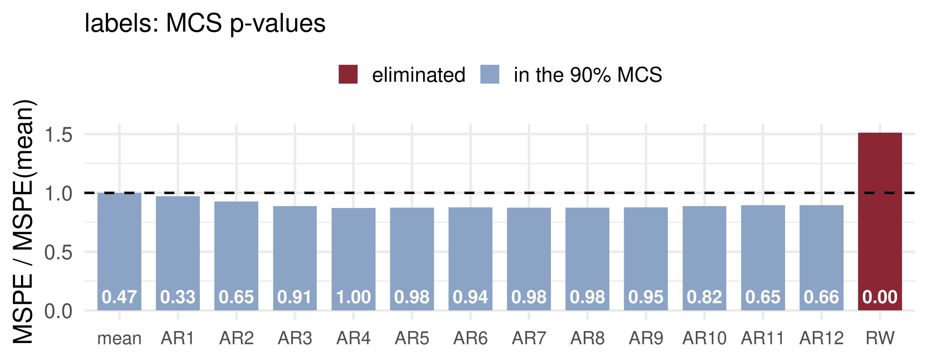
mean  AR1  AR2  AR3  AR4  AR5  AR6  AR7  AR8  AR9 AR10 AR11 AR12   RW 
1.00 0.97 0.93 0.89 0.87 0.87 0.88 0.87 0.87 0.88 0.89 0.90 0.90 1.51 
   p_RC p_SPA MCS90_size
1 0.237 0.129         13
[1] "RW"

Below 1 beats the mean. Compare \(p_{RC}\) and \(p_{SPA}\) with 0.05; the last line lists the models outside the 90% MCS.

💰 Case Study: What the Data Say

What the data say: the AR models cut the MSPE of the mean by up to 13%, yet neither test rejects: 360 months of noisy loss differentials cannot settle a gain that size. SPA’s \(p\)-value sits below the Reality Check’s because the hopeless random walk no longer inflates its critical value. The MCS removes only the random walk.

📝 Quiz #1: Snooping Arithmetic

Ten independent rules, none with skill. What is the probability that the best of them has a one-sided 5% “significant” \(t\)-statistic?

  • \(1 - 0.95^{10} \approx 0.40\)
  • \(0.05\)
  • \(10 \times 0.05 = 0.50\)
  • \(0.05^{10}\)

📝 Quiz #2: The SPA Null

With \(d_{j,t} = L_t^{(0)} - L_t^{(j)}\) (benchmark loss minus competitor loss), what is the null hypothesis of the Reality Check and the SPA test?

  • \(E[d_{j,t}] \le 0\) for every competitor \(j\): no model beats the benchmark
  • \(E[d_{j,t}] = 0\) for some competitor \(j\)
  • \(E[d_{j,t}] > 0\) for every competitor \(j\)
  • \(E[d_{ij,t}] = 0\) for every pair \(i, j\)

📝 Quiz #3: Reading an MCS

A 90% model confidence set from eight volatility models contains six of them. What is the right reading?

  • The data cannot distinguish those six; with probability at least 0.9 the best model is among them
  • The six models are equally good in population
  • The best model is the one with the lowest sample loss among the six
  • Two models are significantly better than the other six

📋 Key Formulas

Best of \(m\) independent nulls \(\Pr(\max_j t_j > c) = 1 - \Phi(c)^m\)
SPA hypotheses \(H_0: \mu_j \le 0\ \forall j\) vs \(H_A: \mu_j > 0\) for some \(j\); \(\mu_j = E[L^{(0)}_t - L^{(j)}_t]\)
Reality Check \(V = \max_j \sqrt P\,\bar d_j\); \(V^* = \max_j \sqrt P(\bar d^*_j - \bar d_j)\)
Hansen SPA studentise by \(\hat\omega_j\); recentre only if \(\sqrt P\bar d_j/\hat\omega_j \ge -\sqrt{2\log\log P}\)
MCS target \(\mathcal M^* = \{i : E[L^{(i)}_t - L^{(j)}_t] \le 0\ \forall j\}\)
MCS membership \(i \in \widehat{\mathcal M}^*_{1-\alpha} \iff \hat p_i \ge \alpha\)

📋 Summary

  • Choosing the best of many models and then testing it as if it had been chosen in advance is data snooping; the best of 100 null models has a 99% chance of looking significant.
  • The Reality Check compares the best model with the bootstrap distribution of the best, under the least favourable null.
  • Hansen’s SPA test studentises and ignores clearly poor models, which gives it more power.
  • The model confidence set answers “which may the best be?” by sequential elimination, with an MCS \(p\)-value for every model.

📚 Further Reading and Next Lecture

  • White (2000), “A reality check for data snooping”, Econometrica.
  • Hansen (2005), “A test for superior predictive ability”, JBES.
  • Hansen, Lunde and Nason (2011), “The model confidence set”, Econometrica.
  • Politis and Romano (1994), “The stationary bootstrap”, JASA.
  • Sullivan, Timmermann and White (1999), on data snooping in technical trading rules.

Next lecture: Linear Projection, Innovations and the Wold Decomposition. We now model the conditional mean itself, starting from the one representation every stationary series has.