Time Series Econometrics

Lecture 9: Trends, Unit Roots and Brownian Motion

Samir Orujov, PhD

Open lecture notes, after Stanislav Anatolyev’s course (2016)

🎬 The Idea in 3 Minutes

⬅ Previous lecture: 8 · ARMA Models: Identification, Estimation, Forecasting

A short film with the intuition. Watch it before the slides, or after. Captions: CC button.

🎯 Learning Objectives

By the end of this lecture, you will be able to:

• Distinguish a deterministic trend from a stochastic trend, and say what each implies for shocks and forecasts
• Derive the OLS rates \(\sqrt T\), \(T^{3/2}\) and \(T\) for a constant, a linear trend and a unit root
• Show by a telescoping sum that \(T(\hat\rho - 1)\) has a non-normal limit, the Dickey–Fuller distribution
• State the properties of Brownian motion and the functional central limit theorem
• Translate sums of a random walk into stochastic integrals, using Itô’s rule where ordinary calculus fails

🔁 Warm-up from last time

For a stationary AR(1), \(x_t = \mu + \rho(x_{t-1} - \mu) + \varepsilon_t\), what happens to the \(h\)-step forecast MSE as \(h \to \infty\)?

• It rises to the unconditional variance \(\sigma^2/(1 - \rho^2)\)
• It stays at \(\sigma^2\) for every \(h\)
• It grows without bound, linearly in \(h\)
• It falls to zero, since the forecast converges to \(\mu\)

🗺️ Where We Are

Lecture 8 ended with two comforting facts about a stationary ARMA: forecasts revert to the mean, and the forecast MSE is bounded by \(\gamma_0\). Both rest on \(|\rho| < 1\).

At \(\rho = 1\) both fail. The forecast of \(y_{T+h}\) is \(y_T\) for every \(h\), and the MSE is \(h\sigma^2\). The asymptotic theory fails as well: OLS is still consistent, but \(\sqrt T\) is the wrong rate and the limit is not normal. Today we find the right rate and the right limit, and the tool that delivers them, Brownian motion.

❓ The Question

Was the 2008 recession a permanent loss?

US real GDP fell about 4% in 2008–09. If output fluctuates around a fixed trend line, it should have caught up with that line. If its trend is itself a random walk, the loss was permanent and the old line is irrelevant.

The two views agree on the past and disagree about the future. Nelson and Plosser (1982) found most US macro series behave like the second. Telling them apart is the problem of unit-root econometrics, and its statistics are non-standard.

Not in the 2016 notes: framing added from Hamilton (1994), ch. 15.

📐 Two Kinds of Trend

	trend-stationary (TS)	difference-stationary (DS)
model	\(y_t = \alpha + \delta t + u_t\)	\(y_t = \delta + y_{t-1} + u_t\)
solved	\(u_t\) stationary around a line	\(y_t = y_0 + \delta t + \sum_{s\le t}u_s\)
a shock	dies out	stays forever
forecast MSE	bounded	grows like \(h\)
made stationary by	detrending	differencing

The DS trend contains a random walk, \(\sum_{s\le t}u_s\): \(y_t\) has a unit root. Detrending does not make it stationary; differencing a TS series creates a non-invertible MA root.

Not in the 2016 notes: added from Hamilton (1994), ch. 15.

💻 Same Drift, Different Memory

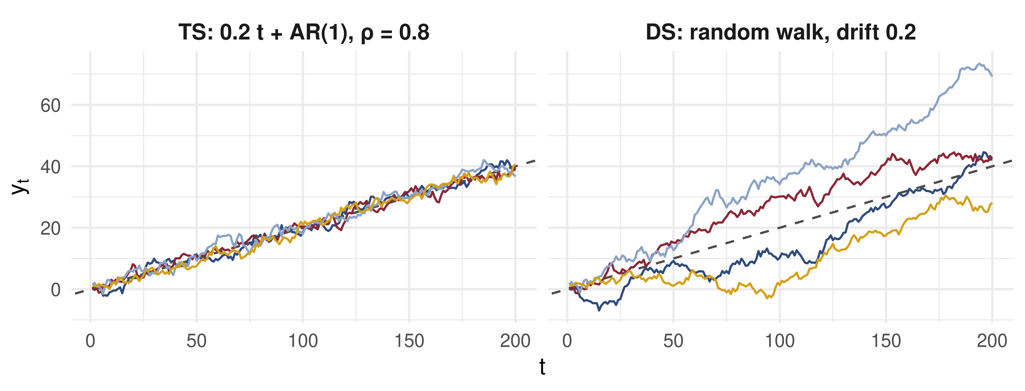
Same shocks in both panels. Left: every path hugs the dashed line. Right: paths wander off and never come back; their spread grows like \(\sqrt t\).

Not in the 2016 notes: added from Hamilton (1994), ch. 15.

📐 Three Regular Models

\(\varepsilon_t\) i.i.d. \((0, \sigma^2)\); each OLS estimator is truth plus error:

model	OLS error	numerator	denominator
\(y_t = \mu + \varepsilon_t\)	\(\hat\mu - \mu = \dfrac{\sum 1\cdot\varepsilon_t}{\sum 1^2}\)	stationary, zero-mean	\(T\)
\(y_t = \rho y_{t-1} + \varepsilon_t\), \(\lvert\rho\rvert < 1\)	\(\hat\rho - \rho = \dfrac{\sum y_{t-1}\varepsilon_t}{\sum y_{t-1}^2}\)	stationary, zero-mean	stationary, mean \(\gamma_0\)
\(y_t = \delta t + \varepsilon_t\)	\(\hat\delta - \delta = \dfrac{\sum t\,\varepsilon_t}{\sum t^2}\)	trended, zero-mean	quadratic trend

Rate of convergence: the power of \(T\) giving a non-degenerate limit. Rows 1–2 have stationary sums: rate \(\sqrt T\), limits \(N(0,\sigma^2)\) and \(N(0,1-\rho^2)\).

✏️ Worked Example: The Linear Trend

\(y_t = \delta t + \varepsilon_t\). The denominator is \(\sum_{t=1}^T t^2 = \frac{T(T+1)(2T+1)}{6}\), so \(\frac{1}{T^3}\sum t^2 \to \frac13\): it grows like \(T^3\).

The numerator has mean 0 and \(\operatorname{Var}\big(\sum t\,\varepsilon_t\big) = \sum t^2 E\varepsilon_t^2 = \sigma^2\sum t^2\), of order \(T^3\): it grows like \(T^{3/2}\). Hence \[T^{3/2}(\hat\delta - \delta) = \frac{T^{-3/2}\sum t\,\varepsilon_t}{T^{-3}\sum t^2}.\]

The numerator is asymptotically normal with variance \(\sigma^2 T^{-3}\sum t^2 \to \sigma^2/3\); the denominator tends to \(1/3\). So \[T^{3/2}(\hat\delta - \delta) \xrightarrow{d} N\Big(0,\ \frac{\sigma^2/3}{(1/3)^2}\Big) = N(0,\ 3\sigma^2).\] The rate is fast, and the \(t\)-statistic is still asymptotically \(N(0,1)\): with a deterministic trend, inference is standard.

📐 The Unit Root: What Changes

\(y_t = \rho y_{t-1} + \varepsilon_t\) with \(\rho = 1\), and \(y_0 = 0\), so \(y_t = \varepsilon_1 + \dots + \varepsilon_t\): \[\hat\rho = 1 + \frac{\sum_{t=1}^T y_{t-1}\varepsilon_t}{\sum_{t=1}^T y_{t-1}^2}.\]

• Numerator and denominator are both sums of stochastically trended terms
• They grow at different rates, neither of them \(T\)
• \(\hat\rho \xrightarrow{p} 1\) still holds, but the speed of convergence is unknown

We find each rate in turn, starting with the numerator.

✏️ The Numerator: A Telescoping Sum

Square the recursion: \(y_t^2 = (y_{t-1} + \varepsilon_t)^2 = y_{t-1}^2 + 2y_{t-1}\varepsilon_t + \varepsilon_t^2\). Sum over \(t\) and solve for the cross term: \[\sum_{t=1}^T y_{t-1}\varepsilon_t = \frac12\Big\{\sum_{t=1}^T\big(y_t^2 - y_{t-1}^2\big) - \sum_{t=1}^T\varepsilon_t^2\Big\}.\]

The first sum telescopes, \((y_T^2 - y_{T-1}^2) + (y_{T-1}^2 - y_{T-2}^2) + \dots = y_T^2 - y_0^2 = y_T^2\). Divide by \(T\): \[\frac1T\sum_{t=1}^T y_{t-1}\varepsilon_t = \frac12\Big\{\Big(\frac{y_T}{\sqrt T}\Big)^2 - \frac1T\sum_{t=1}^T\varepsilon_t^2\Big\} \xrightarrow{d} \frac{\sigma^2}{2}\big\{\chi^2(1) - 1\big\}.\]

Why: by the CLT \(y_T/\sqrt T = T^{-1/2}\sum\varepsilon_t \xrightarrow{d} N(0, \sigma^2)\), so its square tends to \(\sigma^2\chi^2(1)\); by the LLN \(T^{-1}\sum\varepsilon_t^2 \xrightarrow{p} \sigma^2\).

✏️ The Denominator: Order \(T^2\)

\(y_{t-1}\) does not contain \(\varepsilon_t\), and \(\operatorname{Var}(y_{t-1}) = (t-1)\sigma^2\), so \[E\Big[\sum_{t=1}^T y_{t-1}^2\Big] = \sum_{t=1}^T(t-1)\sigma^2 = \sigma^2\,\frac{T(T-1)}{2}:\] the denominator is of order \(T^2\). Divide top and bottom accordingly: \[T(\hat\rho - 1) = \frac{T^{-1}\sum y_{t-1}\varepsilon_t}{T^{-2}\sum y_{t-1}^2} \xrightarrow{d} \frac{\tfrac12\{\chi^2(1) - 1\}}{\text{a random limit}} \overset{d}{=} DF.\]

The rate is \(T\), not \(\sqrt T\): \(\hat\rho\) is superconsistent. The limit, the Dickey–Fuller distribution, is not normal, and numerator and denominator limits are dependent.

💻 Dickey–Fuller by Simulation

Tn <- 500; R <- 10000
e  <- matrix(rnorm(Tn * R), Tn)                 # one column per replication
y  <- apply(e, 2, cumsum)                       # random walks, y_0 = 0
df_stat <- Tn * colSums(y[-Tn, ] * e[-1, ]) / colSums(y[-Tn, ]^2)
q <- quantile(df_stat, c(0.01, 0.05, 0.10))
ggplot(data.frame(s = df_stat), aes(s)) +
  geom_vline(xintercept = q, colour = "#8b2635", linetype = "dotted") +
  geom_histogram(aes(y = after_stat(density)), binwidth = 0.5, fill = "#8ba3c7", colour = "white") +
  geom_vline(xintercept = 0, linetype = "dashed") + coord_cartesian(xlim = c(-20, 6)) +
  labs(x = expression(T(hat(rho) - 1)), y = "density",
       subtitle = sprintf("Dotted: 1%%, 5%%, 10%% quantiles = %.1f, %.1f, %.1f.   Share below 0: %.2f",
                          q[1], q[2], q[3], mean(df_stat < 0))) +
  theme_minimal(base_size = 20)

🔍 Reading the Simulation

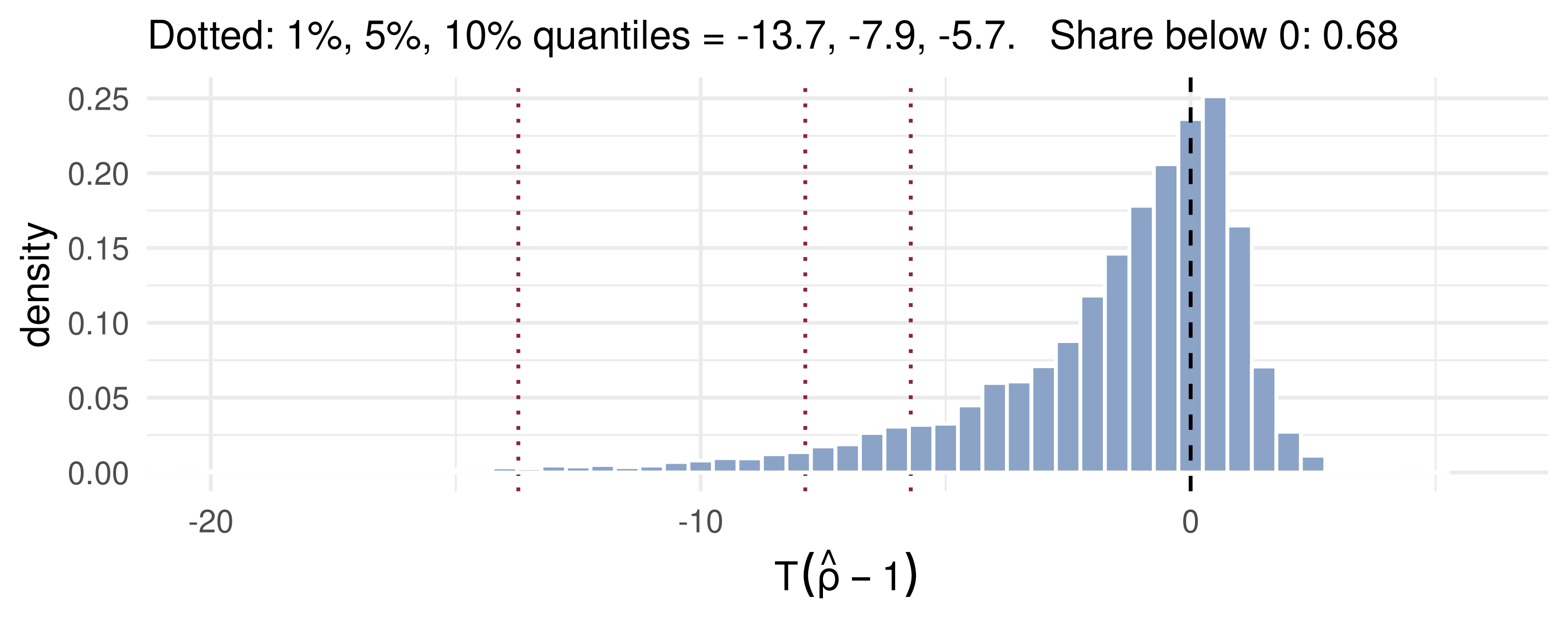
• The 1%, 5% and 10% quantiles match the tabulated asymptotic values for the regression without a constant, \(-13.8\), \(-8.1\), \(-5.7\) (Fuller 1976)
• About two thirds of the estimates fall below 1: \(\hat\rho\) is biased downwards, and the density has a long left tail
• A \(t\)-test of \(\rho = 1\) with normal critical values would reject far too often
• The limit does not depend on \(\sigma^2\): one table serves every application. Next lecture builds the tests on it

💻 Three Rates in One Picture

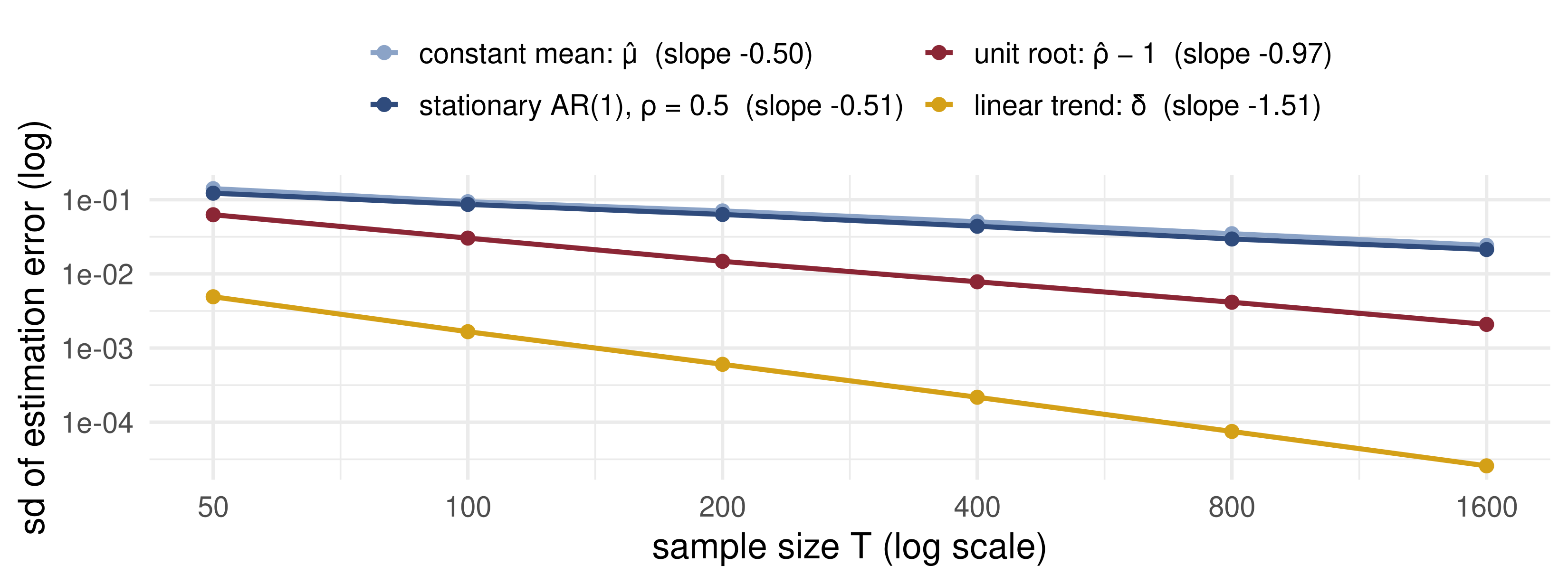
On log–log axes a rate \(T^{a}\) is a line of slope \(-a\): \(-\tfrac12\) for the constant and the stationary AR, \(-1\) for the unit root, \(-\tfrac32\) for the trend.

📐 Rescaling a Random Walk

Let \(\varepsilon_t\) be strong white noise and \(S_t = \sum_{s=1}^t\varepsilon_s\). As \(T\) grows, \(S_T\) spreads out like \(\sigma\sqrt T\). To see a limit we shrink both axes:

• height by \(\sigma\sqrt T\), so the end point has variance 1
• time by \(T\), so the walk lives on the fixed interval \([0, 1]\)

\[S_T(r) = \frac{1}{\sigma\sqrt T}\,S_{\lfloor Tr\rfloor}, \qquad r \in [0, 1],\] where \(\lfloor\cdot\rfloor\) is the integer part. \(S_T(r)\) is a random function, a step function with \(T\) steps of height \(\pm\varepsilon_t/(\sigma\sqrt T)\).

🎛️ Explore: Shrinking the Steps

viewof logT = Inputs.range([1, 4], {step: 0.25, value: 1, label: "log₁₀ T"})

coin = {
  let s = 777;                                         // fixed seed: one sequence of ±1 steps
  return Array.from({length: 10000}, () => { s = (s * 16807) % 2147483647; return s / 2147483647 < 0.5 ? -1 : 1; });
}

walk = {
  const T = Math.round(Math.pow(10, logT)), out = [];
  let S = 0;                                           // S_T(r) = S_floor(Tr) / sqrt(T): flat on [t/T, (t+1)/T)
  for (let t = 0; t < T; t++) { out.push({r: t / T, S: S / Math.sqrt(T)}); out.push({r: (t + 1) / T, S: S / Math.sqrt(T)}); S += coin[t]; }
  out.push({r: 1, S: S / Math.sqrt(T)});
  return out;
}

Plot.plot({
  width: 1100, height: 320, marginLeft: 70, marginBottom: 55, marginTop: 30, style: {fontSize: "18px"},
  x: {label: "r", domain: [0, 1]}, y: {label: "S_T(r)", domain: [-3, 3]}, clip: true,
  marks: [
    Plot.ruleY([0], {stroke: "#bbb"}),
    Plot.line(d3.range(0, 1.001, 0.01), {x: r => r, y: r => 1.96 * Math.sqrt(r), stroke: "#8ba3c7", strokeDasharray: "6,4"}),
    Plot.line(d3.range(0, 1.001, 0.01), {x: r => r, y: r => -1.96 * Math.sqrt(r), stroke: "#8ba3c7", strokeDasharray: "6,4"}),
    Plot.line(walk, {x: "r", y: "S", stroke: "#8b2635", strokeWidth: 1.6})
  ]
})

Fair-coin steps of \(\pm1\), rescaled. At \(T = 10\) it is a staircase; at \(T = 10^4\) it looks like Brownian motion. Dashes: \(\pm1.96\sqrt r\), the 95% band of \(N(0, r)\).

📐 Brownian Motion

Definition (standard Brownian motion, or Wiener process, \(B(r)\) on \([0,1]\))

1. \(B(0) = 0\).
2. For \(0 \le r_1 < r_2 < \dots < r_k \le 1\), the increments \(B(r_1)\), \(B(r_2) - B(r_1)\), …, \(B(1) - B(r_k)\) are independent.
3. For \(0 \le r_1 \le r_2 \le 1\): \(\ B(r_2) - B(r_1) \sim N(0,\ r_2 - r_1)\).

It is the continuous-time random walk. Its paths are continuous everywhere and differentiable nowhere: \(\{B(r + h) - B(r)\}/h\) has standard deviation \(1/\sqrt h \to \infty\). And it is Gaussian, although the \(\varepsilon_t\) need not be.

📐 The Functional CLT

Theorem (FCLT, Donsker’s invariance principle)

If \(\varepsilon_t\) is i.i.d. \((0, \sigma^2)\), then \[S_T(r) = \frac{1}{\sigma\sqrt T}\,S_{\lfloor Tr\rfloor} \xrightarrow{d} B(r)\] as random functions on \([0, 1]\).

• At \(r = 1\) it is the ordinary CLT: \(S_T(1) = \frac{1}{\sigma\sqrt T}\sum\varepsilon_t \xrightarrow{d} N(0, 1)\)
• It says more: the whole path converges, so every continuous functional of the path converges too (continuous mapping theorem)
• That is what turns sums of a random walk into integrals of \(B\)

🧠 Think-Pair-Share

\(y_t = y_{t-1} + \varepsilon_t\), \(y_0 = 0\), \(\varepsilon_t\) i.i.d. \((0, \sigma^2)\).

1. By what power of \(T\) must \(\sum_{t=1}^T y_{t-1}\) be divided to converge? To what?
2. Same question for \(\sum_{t=1}^T t\,\varepsilon_t\).
3. Use \(\operatorname{Var}\int_0^1 r\,dB(r) = \int_0^1 r^2\,dr\) to find the variance of the limit in 2. Have you seen that number before?

✅ Think-Pair-Share: Solution

1. \(y_{t-1} \to \sigma\sqrt T\,B(r)\) and \(1 \to T\,dr\): the sum carries \(\sigma T^{3/2}\), so \[T^{-3/2}\sum y_{t-1} \xrightarrow{d} \sigma\int_0^1 B(r)\,dr \ \sim N(0, \sigma^2/3).\]

2. \(t \to T r\) and \(\varepsilon_t \to \sigma\sqrt T\,dB(r)\): again \(T^{3/2}\), and \[T^{-3/2}\sum t\,\varepsilon_t \xrightarrow{d} \sigma\int_0^1 r\,dB(r).\]

3. Variance \(\sigma^2\int_0^1 r^2dr = \sigma^2/3\): exactly the numerator variance of the linear-trend example, where we found \(T^{3/2}(\hat\delta - \delta) \to N(0, 3\sigma^2)\). The mnemonics reproduce it.

📐 Corollaries of the FCLT

\[\begin{aligned} T^{-1/2}\textstyle\sum\varepsilon_t &\xrightarrow{d} \sigma\int_0^1 dB(r) = \sigma B(1) \sim N(0, \sigma^2)\\ T^{-1}\textstyle\sum y_{t-1}\varepsilon_t &\xrightarrow{d} \sigma^2\int_0^1 B(r)\,dB(r)\\ T^{-2}\textstyle\sum y_{t-1}^2 &\xrightarrow{d} \sigma^2\int_0^1 B(r)^2\,dr\\ T^{-2}\textstyle\sum t\,y_{t-1}\varepsilon_t &\xrightarrow{d} \sigma^2\int_0^1 r\,B(r)\,dB(r) \end{aligned}\]

Mnemonics: \(\ \sum_{t=1}^T \to \int_0^1\); \(\ \varepsilon_t \to dB(r)\) and \(y_{t-1} \to B(r)\), factor \(\sigma\sqrt T\) each; \(\ 1 \to dr\) and \(t \to r\), factor \(T\) each. The product of the factors is the normalisation: \(T \cdot \sigma\sqrt T \cdot \sigma\sqrt T = \sigma^2T^2\) in the last line.

⚠️ The Trap: \(\int B\,dB\)

Ordinary calculus would say \(\int_0^1 B\,dB = \tfrac12\int_0^1 d(B^2) = \tfrac12 B(1)^2\). This is wrong for Brownian motion.

Increments of \(B\) are of size \(\sqrt{dr}\), so \((dB)^2\) is of order \(dr\), not negligible. Itô’s rule keeps it: \[d(B^2) = 2B\,dB + dr \quad\Longrightarrow\quad \int_0^1 B(r)\,dB(r) = \tfrac12\big\{B(1)^2 - 1\big\}.\]

This agrees with the telescoping sum: \(T^{-1}\sum y_{t-1}\varepsilon_t \to \tfrac{\sigma^2}{2}\{B(1)^2 - 1\} \overset{d}{=} \tfrac{\sigma^2}{2}\{\chi^2(1) - 1\}\). The “\(-1\)” is the \(T^{-1}\sum\varepsilon_t^2\) term, which is exactly what \((dB)^2 = dr\) accounts for.

💻 Itô’s Correction, Numerically

n <- 1000; R <- 2000                          # grid of n steps on [0, 1]
dB <- matrix(rnorm(n * R, sd = sqrt(1 / n)), n)
B  <- apply(dB, 2, cumsum); Bprev <- rbind(0, B[-n, ])
ito  <- colSums(Bprev * dB)                   # left-point sum: sum B(r_{i-1}) dB_i
B1   <- B[n, ]
qv   <- colSums(dB^2)                         # quadratic variation
round(c(mean_ito = mean(ito), mean_naive = mean(B1^2 / 2), mean_ito_formula = mean((B1^2 - 1) / 2),
        mean_quadratic_variation = mean(qv), max_gap_to_formula = max(abs(ito - (B1^2 - 1) / 2))), 3)

                mean_ito               mean_naive         mean_ito_formula 
                  -0.008                    0.493                   -0.007 
mean_quadratic_variation       max_gap_to_formula 
                   1.001                    0.073 

The sum has mean 0, as \(\tfrac12\{B(1)^2 - 1\}\) does; the naive \(\tfrac12B(1)^2\) has mean \(\tfrac12\). The gap is the quadratic variation \(\sum(\Delta B)^2 \approx 1\).

📐 The Dickey–Fuller Limit

Combine the second and third corollaries. The \(\sigma^2\) cancels: \[T(\hat\rho - 1) = \frac{T^{-1}\sum y_{t-1}\varepsilon_t}{T^{-2}\sum y_{t-1}^2} \xrightarrow{d} \frac{\int_0^1 B(r)\,dB(r)}{\int_0^1 B(r)^2\,dr} = \frac{\tfrac12\{B(1)^2 - 1\}}{\int_0^1 B(r)^2\,dr}.\]

• The “random limit” of the denominator is \(\int_0^1 B(r)^2\,dr\)
• Numerator and denominator are functionals of the same path, hence dependent
• The law is free of nuisance parameters but non-standard: its quantiles come from simulation, as on our earlier slide

💰 Case Study: US Output After 2008

📈 The question

1. Fitted as TS, how persistent are the deviations from trend?
2. From the 2009Q2 trough, what do the TS and DS models forecast for 2026?
3. Which forecast was closer?

📊 The data

Series: real GDP, FRED GDPC1, quarterly

Estimation: 1947Q1 – 2007Q4; forecast: 2009Q3 – 2026Q2

Transformation: \(y_t = 100\log\text{GDP}_t\)

read.csv("https://fred.stlouisfed.org/
  graph/fredgraph.csv?id=GDPC1")

💰 Case Study: TS vs DS

g  <- read.csv("data/GDPC1.csv"); g$date <- as.Date(g$observation_date)
y  <- 100 * log(g$GDPC1); tt <- seq_along(y)
est <- g$date <= as.Date("2007-10-01"); n <- sum(est)
ts_fit <- lm(y[est] ~ tt[est]); u <- resid(ts_fit)          # TS: line + AR(1) deviation
rho_u  <- unname(coef(lm(u[-1] ~ u[-n] - 1)))
g_hat  <- mean(diff(y[est]))                                 # DS: mean quarterly growth
o <- which(g$date == as.Date("2009-04-01")); h <- 1:(length(y) - o)
u_o <- y[o] - sum(coef(ts_fit) * c(1, o))
ts_fc <- sum(coef(ts_fit) * c(1, 0)) + coef(ts_fit)[2] * (o + h) + rho_u^h * u_o
ds_fc <- y[o] + g_hat * h; last <- length(h)
round(c(trend_growth = unname(coef(ts_fit)[2]), rho_deviation = rho_u, T_rho_minus_1 = n * (rho_u - 1),
        gap_to_trend_2009Q2 = u_o, error_TS_2026Q2 = y[o + last] - unname(ts_fc[last]),
        error_DS_2026Q2 = y[o + last] - ds_fc[last]), 2)

       trend_growth       rho_deviation       T_rho_minus_1 gap_to_trend_2009Q2 
               0.84                0.97               -6.80              -14.27 
    error_TS_2026Q2     error_DS_2026Q2 
             -28.80              -16.74 

Growth is in log points per quarter; errors are actual minus forecast, in log points (≈ %).

💰 Case Study: The Lost Trend

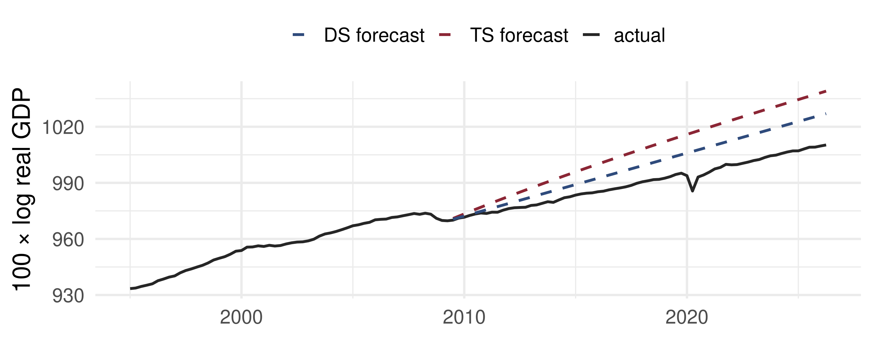
What the data say: GDP never returned to its old trend line: the TS forecast (back to the 1947–2007 line) misses by about 29%, the DS forecast (drift from the trough) by 17%. Deviations from trend have AR coefficient 0.97, and \(T(\hat\rho - 1) \approx -6.8\) is far from the detrended 5% Dickey–Fuller value, about \(-21.8\) (next lecture). DS overpredicts too: growth after 2009 fell below the old drift.

📝 Quiz #1: Rates

In \(y_t = \delta t + \varepsilon_t\) with i.i.d. errors, which normalisation gives \(\hat\delta\) a non-degenerate normal limit?

• \(T^{3/2}(\hat\delta - \delta)\)
• \(\sqrt T(\hat\delta - \delta)\)
• \(T(\hat\delta - \delta)\)
• \(T^2(\hat\delta - \delta)\)

📝 Quiz #2: Itô

Which is \(\int_0^1 B(r)\,dB(r)\) for standard Brownian motion?

• \(\tfrac12\{B(1)^2 - 1\}\)
• \(\tfrac12B(1)^2\)
• \(B(1)\)
• \(\int_0^1 B(r)^2dr\)

📝 Quiz #3: Brownian Increments

What is the distribution of \(B(0.7) - B(0.2)\), and how does it relate to \(B(0.2)\)?

• \(N(0, 0.5)\), independent of \(B(0.2)\)
• \(N(0, 0.5)\), positively correlated with \(B(0.2)\)
• \(N(0, 0.7)\), independent of \(B(0.2)\)
• \(N(0, 0.25)\), independent of \(B(0.2)\)

📋 Key Formulas

Constant mean	\(\sqrt T(\hat\mu - \mu) \to N(0, \sigma^2)\)
Stationary AR(1)	\(\sqrt T(\hat\rho - \rho) \to N(0, 1 - \rho^2)\)
Linear trend	\(T^{3/2}(\hat\delta - \delta) \to N(0, 3\sigma^2)\)
Telescoping	\(\sum y_{t-1}\varepsilon_t = \tfrac12\{y_T^2 - \sum\varepsilon_t^2\}\)
Unit root	\(T(\hat\rho - 1) \to \dfrac{\tfrac12\{B(1)^2 - 1\}}{\int_0^1 B^2dr}\)
Brownian motion	\(B(0) = 0\), independent increments, \(B(r_2) - B(r_1) \sim N(0, r_2 - r_1)\)
FCLT	\(\frac{1}{\sigma\sqrt T}S_{\lfloor Tr\rfloor} \to B(r)\)
Itô	\(\int_0^1 B\,dB = \tfrac12\{B(1)^2 - 1\}\)

📋 Summary

• A deterministic trend changes the rate (\(T^{3/2}\)) but not the normality of OLS: \(t\)-tests remain valid
• A stochastic trend changes both: \(T(\hat\rho - 1)\) has the Dickey–Fuller limit, biased left and skewed left
• The FCLT turns a rescaled random walk into Brownian motion; sums become integrals by the mnemonics
• \(\int B\,dB = \tfrac12\{B(1)^2 - 1\}\), not \(\tfrac12B(1)^2\)
• US GDP after 2008 behaved like a DS series: the lost output was not recovered

📚 Further Reading

• Hamilton, J. D. (1994). Time Series Analysis. Princeton. Ch. 15 (trends), ch. 16 (deterministic trends), ch. 17 (unit roots, FCLT)
• Tsay, R. S. (2010). Analysis of Financial Time Series, 3rd ed. Wiley. §2.7
• Nelson, C. R. and Plosser, C. I. (1982). Trends and random walks in macroeconomic time series. Journal of Monetary Economics 10, 139–162
• Phillips, P. C. B. (1987). Time series regression with a unit root. Econometrica 55, 277–301
• Fuller, W. A. (1976). Introduction to Statistical Time Series. Wiley

Next lecture: Dickey–Fuller, Phillips–Perron and ADF Tests.