Time Series Econometrics

Lecture 10: Dickey–Fuller, Phillips–Perron and ADF Tests

Samir Orujov, PhD

Open lecture notes, after Stanislav Anatolyev’s course (2016)

🎬 The Idea in 3 Minutes

⬅ Previous lecture: 9 · Trends, Unit Roots and Brownian Motion

A short film with the intuition. Watch it before the slides, or after. Captions: CC button.

🎯 Learning Objectives

By the end of this lecture, you will be able to:

• Derive the Dickey–Fuller limit of \(T(\hat\rho-1)\) from the FCLT, and explain why it is pivotal

• Carry out the DF test with the right deterministic terms and the right critical values

• Correct for serially correlated errors, nonparametrically (Phillips–Perron) or parametrically (ADF)

• Interpret a unit-root verdict as a statement about the persistence of shocks, and its limits

🔁 Warm-up from last time

Lecture 9: \(y_t=y_{t-1}+\varepsilon_t\), \(y_0=0\), \(\varepsilon_t\) i.i.d.\((0,\sigma^2)\). What is the limit of \(\frac1T\sum_{t=1}^T y_{t-1}\varepsilon_t\)?

• \(\frac{\sigma^2}{2}\{\chi^2(1)-1\}\)
• \(N(0,\sigma^4)\), as in the stationary case
• \(0\), because \(E(y_{t-1}\varepsilon_t)=0\)
• \(\frac{\sigma^2}{2}\chi^2(1)\)

🗺️ Where We Are

Lecture 9 ended on a limit: \[T(\hat\rho-1)\ \xrightarrow{d}\ \frac{\int_0^1 \mathcal B\,d\mathcal B}{\int_0^1 \mathcal B(r)^2dr}.\] It is non-normal, skewed to the left, and free of \(\sigma^2\).

Today that limit becomes a test. Three questions decide whether the test is usable in practice: which deterministic terms enter the regression, what to do when the errors are serially correlated, and what a rejection or non-rejection actually tells us.

❓ The Question

Are recessions forgotten?

US real GDP fell about 4% in 2008–09. Does log GDP return to its old trend line, or is the loss carried forward for ever?

If log GDP is trend-stationary, a shock dies out and the old path returns. If it has a unit root, every shock shifts the whole future path, and “returning to trend” has no meaning. The two views give the same short-run forecasts and very different long-run ones.

📐 Random-Walk Moments (FCLT)

Let \(\varepsilon_t\) be white noise with variance \(\sigma^2\) and \(x_t=x_{t-1}+\varepsilon_t\). With \(S_T(r)=\frac{1}{\sigma\sqrt T}\,x_{[Tr]}\), \[S_T(r)\ \Rightarrow\ \mathcal B(r)\quad\text{(standard Brownian motion on }[0,1]),\] \[\frac1T\sum_{t=2}^{T}x_{t-1}\varepsilon_t\ \xrightarrow{d}\ \sigma^2\!\int_0^1\!\mathcal B\,d\mathcal B,\qquad \frac1{T^2}\sum_{t=2}^{T}x_{t-1}^2\ \xrightarrow{d}\ \sigma^2\!\int_0^1\!\mathcal B(r)^2dr,\] jointly.

• Remark 1. The same holds for weak white noise that is a martingale difference sequence; the limit still has independent increments.
• Remark 2. It holds for \(x_0\neq0\), even random, provided \(x_0\) is bounded in probability.

📐 OLS Under a Unit Root

Model \(x_t=\rho x_{t-1}+\varepsilon_t\) with \(\rho=1\). The OLS estimator is \[\hat\rho=\frac{\sum_{t=2}^{T}x_tx_{t-1}}{\sum_{t=2}^{T}x_{t-1}^2}=1+\frac{\sum_{t=2}^{T}x_{t-1}\varepsilon_t}{\sum_{t=2}^{T}x_{t-1}^2}.\]

Scale the numerator by \(T\) and the denominator by \(T^2\): \[T(\hat\rho-1)=\frac{\frac1T\sum x_{t-1}\varepsilon_t}{\frac1{T^2}\sum x_{t-1}^2}\ \xrightarrow{d}\ \underbrace{\frac{\int_0^1\mathcal B\,d\mathcal B}{\int_0^1\mathcal B(r)^2\,dr}}_{DF\ \text{distribution}}.\] The \(\sigma^2\) cancels. The rate is \(T\), not \(\sqrt T\): \(\hat\rho\) is superconsistent.

📐 Pivotal, and Skewed to the Left

Compare the stationary case, \(|\rho|<1\): \[\sqrt T(\hat\rho-\rho)\ \xrightarrow{d}\ N(0,\,1-\rho^2).\] This limit depends on \(\rho\): it is non-pivotal, and we must standardise before tabulating.

The DF distribution contains no unknown parameter: it is pivotal, and can be tabulated once, by simulation.

Its shape: the numerator is \(\int_0^1\mathcal B\,d\mathcal B=\tfrac12\{\mathcal B(1)^2-1\}\), and the denominator is positive, so \[P\big(T(\hat\rho-1)<0\big)\to P\big(\chi^2(1)<1\big)\approx0.68.\] Two thirds of the mass lies below zero: \(\hat\rho\) is biased downwards.

📐 The Dickey–Fuller Test

\[H_0:\ \rho=1\ \text{(unit root)}\qquad\text{vs}\qquad H_A:\ \rho<1\ \text{(stationarity)}\]

The test is one-sided and left-tailed. Two statistics:

• the coefficient statistic: reject \(H_0\) if \(T(\hat\rho-1)<q_\alpha^{DF}\);
• the \(t\)-ratio, \[\tau=\frac{\hat\rho-1}{SE(\hat\rho)}\ \xrightarrow{d}\ \frac{\int_0^1\mathcal B\,d\mathcal B}{\big(\int_0^1\mathcal B(r)^2dr\big)^{1/2}}=DF_\tau ,\] and reject if \(\tau<q_\alpha^{DF_\tau}\).

\(\tau\) is the ordinary OLS \(t\)-statistic. Only its reference distribution changes: \(DF_\tau\), not \(N(0,1)\).

💻 Simulating the DF Distributions

df_stats <- function(x, det) {             # returns T(rho_hat - 1) and tau
  y <- x[-1]; xl <- x[-length(x)]; n <- length(y)
  X <- switch(det, none  = cbind(xl), const = cbind(1, xl),
                   trend = cbind(1, seq_len(n), xl))
  fit <- .lm.fit(X, y); k <- ncol(X); b <- fit$coefficients[k]
  se  <- sqrt(sum(fit$residuals^2) / (n - k) * solve(crossprod(X))[k, k])
  c(n * (b - 1), (b - 1) / se)
}
T <- 500; R <- 10000
sims <- t(replicate(R, { x <- cumsum(rnorm(T))
  c(df_stats(x, "none"), df_stats(x, "const"), df_stats(x, "trend")) }))
colnames(sims) <- c("rho_none", "tau_none", "rho_const", "tau_const",
                    "rho_trend", "tau_trend")
round(apply(sims, 2, quantile, c(0.01, 0.05, 0.10)), 2)
mean(sims[, "rho_none"] < 0)               # theory: P(chi2(1) < 1) = 0.683

    rho_none tau_none rho_const tau_const rho_trend tau_trend
1%    -14.07    -2.63    -20.10     -3.42    -27.88     -3.96
5%     -7.86    -1.93    -13.88     -2.87    -21.47     -3.42
10%    -5.57    -1.60    -11.21     -2.59    -17.96     -3.13
[1] 0.6834

📊 DF Is Not N(0,1)

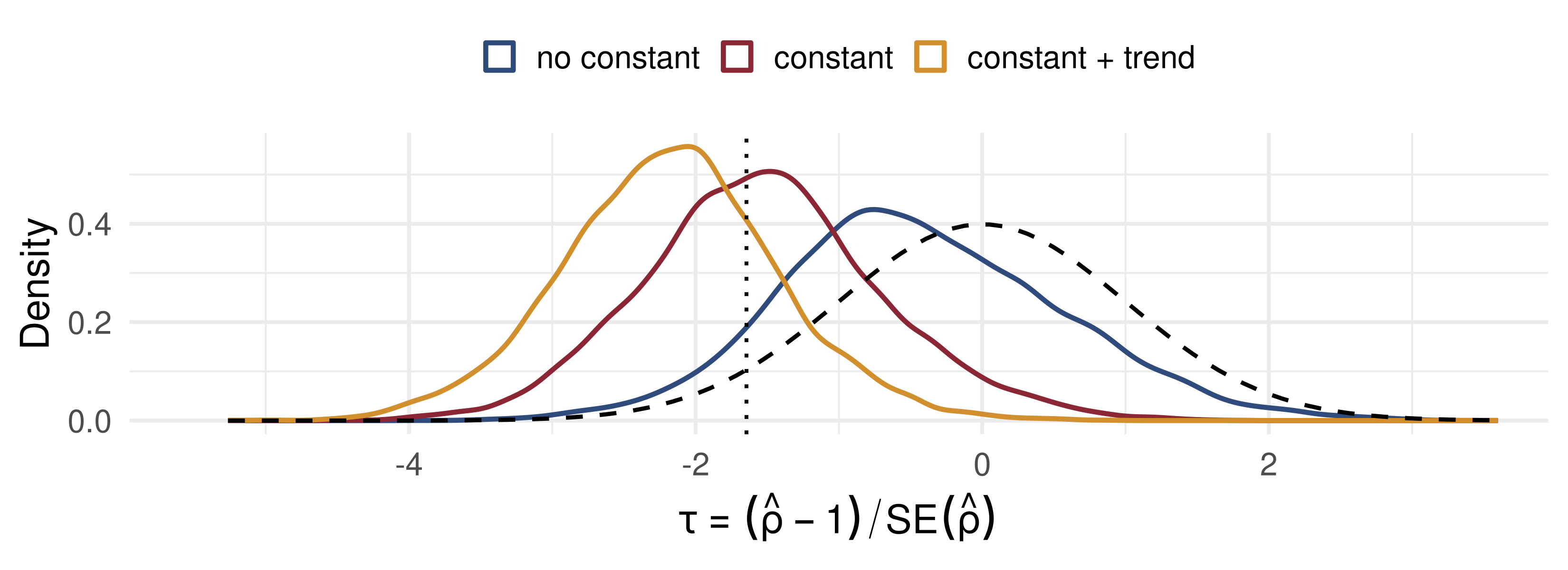
Dashed: \(N(0,1)\); dotted: its 5% point, \(-1.645\). Each DF density lies left of the normal, further left with each deterministic term.

📐 Adding a Constant

Regress \(x_t=\mu+\rho x_{t-1}+\varepsilon_t\) by OLS, obtaining \((\hat\mu,\hat\rho)\). Under \(\rho=1\), \[T(\hat\rho-1)\ \xrightarrow{d}\ \frac{\int_0^1\bar{\mathcal B}(r)\,d\bar{\mathcal B}(r)}{\int_0^1\bar{\mathcal B}(r)^2\,dr}=\overline{DF}, \qquad \bar{\mathcal B}(r)=\mathcal B(r)-\int_0^1\mathcal B(s)\,ds .\]

\(\bar{\mathcal B}\) is the demeaned Brownian motion: estimating \(\mu\) is the continuous-time analogue of subtracting the sample mean from \(x_{t-1}\).

The limit depends on which deterministic terms are in the regression, never on their true values. It is again pivotal.

📐 Adding a Trend

Regress \(x_t=\mu+\delta t+\rho x_{t-1}+\varepsilon_t\), obtaining \((\hat\mu,\hat\delta,\hat\rho)\). Under \(\rho=1\), \[T(\hat\rho-1)\ \xrightarrow{d}\ \frac{\int_0^1\tilde{\mathcal B}(r)\,d\tilde{\mathcal B}(r)}{\int_0^1\tilde{\mathcal B}(r)^2\,dr}=\widetilde{DF}, \qquad \tilde{\mathcal B}(r)=\mathcal B(r)-b_0-b_1r,\] \[\begin{pmatrix}b_0\\ b_1\end{pmatrix}=\begin{pmatrix}\int_0^1(4-6r)\,\mathcal B(r)\,dr\\[2pt] \int_0^1(12r-6)\,\mathcal B(r)\,dr\end{pmatrix}.\]

\(b_0+b_1r\) is the least-squares projection of \(\mathcal B\) on \(\{1,r\}\) in \(L^2[0,1]\): \(\tilde{\mathcal B}\) is \(\mathcal B\) with its own best-fitting line removed.

📋 Critical Values

Asymptotic critical values (MacKinnon, 1996), left tail:

	\(T(\hat\rho-1)\), 1%	5%	10%	\(\tau\), 1%	5%	10%
\(DF\): no constant	−13.8	−8.1	−5.7	−2.57	−1.94	−1.62
\(\overline{DF}\): constant	−20.7	−14.1	−11.3	−3.43	−2.86	−2.57
\(\widetilde{DF}\): + trend	−29.5	−21.8	−18.3	−3.96	−3.41	−3.13

The simulation two slides back, with \(T=500\), reproduces each entry to within about 0.5 for \(T(\hat\rho-1)\) and 0.05 for \(\tau\). More deterministic terms push the critical values further left.

🔧 Which Deterministic Terms?

• Always include a constant, unless the mean has already been removed from the series.
• A trend depends on the situation: include it when the series trends, so that the stationary alternative is “stationary around a line”.

Do not include a time trend	Include a time trend
inflation, unemployment, interest rates, exchange rates	log GNP, log industrial production, log prices

Leaving a trend out of a trending series biases the test towards the unit root. Adding one needlessly costs power.

✍️ Worked Example: A DF Regression

Quarterly log real GDP, \(T=200\). With a constant and a trend, OLS gives \(\hat\rho=0.9620\), \(SE(\hat\rho)=0.0175\).

Step 1. Coefficient statistic: \(T(\hat\rho-1)=200\times(-0.0380)=-7.6\).

Step 2. \(t\)-ratio: \(\tau=-0.0380/0.0175=-2.17\).

Step 3. Compare with the constant + trend row: \(-7.6>-21.8\) and \(-2.17>-3.41\). Do not reject the unit root at 5%.

The trap. Against \(N(0,1)\), \(\tau=-2.17<-1.645\) would “reject”. The normal table overstates the evidence against a unit root.

📐 Serially Correlated Errors

Return to \(x_t=\rho x_{t-1}+u_t\), \(\rho=1\). If the true process is not a random walk, \(u_t=\Delta x_t\) is serially correlated. Write \[\Gamma_j=E(u_tu_{t-j}),\qquad \omega^2=\sum_{j=-\infty}^{\infty}\Gamma_j,\qquad \lambda=\sum_{j=1}^{\infty}\Gamma_j=\frac{\omega^2-\Gamma_0}{2}.\]

With \(\mathcal B\) now the Brownian motion from the FCLT normalised by \(\omega\), \[T(\hat\rho-1)\ \xrightarrow{d}\ \frac{\int_0^1\mathcal B\,d\mathcal B+\lambda/\omega^2}{\int_0^1\mathcal B(r)^2\,dr}.\] The extra term depends on nuisance parameters, so the DF tables no longer apply.

📐 Two Remedies

Nonparametric: Phillips–Perron. Subtract the bias directly: \[Z=T(\hat\rho-1)-\frac{\hat\lambda}{\frac1{T^2}\sum x_{t-1}^2}\ \xrightarrow{d}\ DF .\] \(\hat\lambda=(\hat\omega^2-\hat\Gamma_0)/2\) uses a Newey–West estimate \(\hat\omega^2\). A one-sided sum need not be positive, so no positive-definite estimate of \(\lambda\) is required.

Parametric: augmented Dickey–Fuller. Add lagged differences: \[x_t=\rho x_{t-1}+\sum_{j=1}^{p}\alpha_j\,\underbrace{\Delta x_{t-j}}_{\text{stationary}}+\underbrace{\varepsilon_t}_{\text{pre-whitened}} .\] Choose \(p\) by BIC. Then \(ADF=\dfrac{T(\hat\rho-1)}{1-\sum_j\hat\alpha_j}\xrightarrow{d}DF\), and the \(t\)-ratio on \(\rho\) \(\xrightarrow{d}DF_\tau\).

💻 Does the Correction Work?

nw_lrv <- function(u, L = floor(4 * (length(u) / 100)^(2 / 9))) {
  n <- length(u); g <- sapply(0:L, function(j) sum(u[(j + 1):n] * u[1:(n - j)]) / n)
  g[1] + 2 * sum((1 - (1:L) / (L + 1)) * g[-1])            # Bartlett kernel
}
stats3 <- function(x, pmax = 8) {          # all with a constant
  y <- x[-1]; xl <- x[-length(x)]; n <- length(y)
  f <- .lm.fit(cbind(1, xl), y); dfz <- n * (f$coefficients[2] - 1)
  lam <- (nw_lrv(f$residuals) - mean(f$residuals^2)) / 2
  pp <- dfz - lam / (sum((xl - mean(xl))^2) / n^2)
  dx <- diff(x); fitp <- function(p, i) { X <- cbind(x[i - 1], 1)
    if (p > 0) for (j in 1:p) X <- cbind(X, dx[i - 1 - j]); .lm.fit(X, x[i]) }
  i0 <- (pmax + 2):length(x)
  bic <- sapply(0:pmax, function(p) length(i0) * log(mean(fitp(p, i0)$residuals^2)) + (p + 2) * log(length(i0)))
  p <- which.min(bic) - 1; i <- (p + 2):length(x); b <- fitp(p, i)$coefficients
  adf <- length(i) * (b[1] - 1) / (1 - if (p > 0) sum(b[3:(p + 2)]) else 0)
  c(DF = dfz, PP = pp, ADF = adf)
}
rate <- function(theta, R = 2000, T = 200) { r <- t(replicate(R, {
  e <- rnorm(T + 1); stats3(cumsum(e[-1] + theta * e[-(T + 1)])) }))
  round(colMeans(r < -14.1), 3) }               # -14.1 = 5% point of DF-bar
rbind(`theta = -0.5` = rate(-0.5), `theta = 0` = rate(0), `theta = +0.5` = rate(0.5))

                DF    PP   ADF
theta = -0.5 0.664 0.439 0.182
theta = 0    0.044 0.052 0.045
theta = +0.5 0.002 0.029 0.076

Under \(H_0\) every entry should be 0.05. Uncorrected DF fails badly; ADF comes closest.

🧠 Think–Pair–Share

Two processes, driven by the same shocks, \(T=300\): \[\text{(A)}\ x_t=x_{t-1}+\varepsilon_t,\qquad \text{(B)}\ x_t=0.999\,x_{t-1}+\varepsilon_t .\]

1. After a unit shock, how much remains in (B) after 10 periods? After 700?
2. Would a DF test at 5% tell (A) and (B) apart? Guess the rejection rate under (B).
3. Which of the two do you want for a 4-quarter GDP forecast? For a 50-year pension forecast?

✅ Think–Pair–Share: Solution

1. In (B) the impulse response is \(0.999^h\): \(0.999^{10}=0.990\), \(0.999^{700}=0.496\). The half-life is \(\ln 0.5/\ln 0.999\approx693\) periods. In (A) the whole shock remains for ever.

2. No. With \(T=300\) the two are practically indistinguishable; the rejection rate under (B) is barely above the 5% size (next slide).

3. For four quarters it does not matter: short-run forecasts coincide. For fifty years it matters entirely: (B) reverts to its mean, (A) never does.

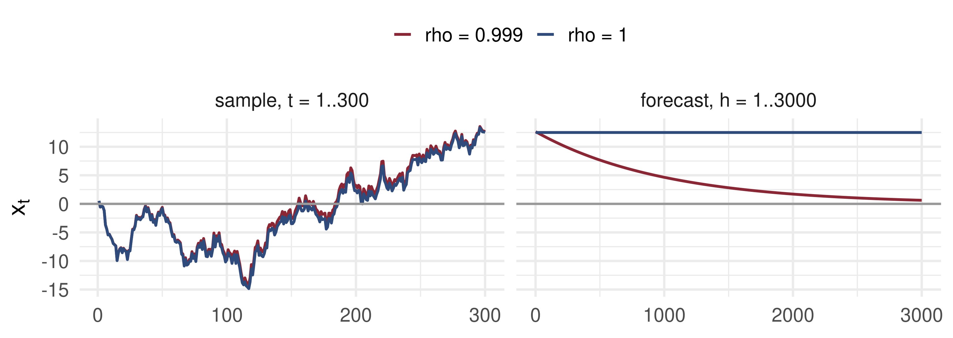
📈 The Twins: ρ = 1 and ρ = 0.999

Same shocks. In the sample the two paths are one line; only the forecasts part company.

📊 Can a Test Tell Them Apart?

rej <- function(rho, R = 2000) mean(replicate(R, {
  x <- as.numeric(stats::filter(rnorm(300), rho, method = "recursive"))
  df_stats(x, "const")[2] < -2.86 }))
c(`rho = 1` = rej(1), `rho = 0.999` = rej(0.999), `rho = 0.95` = rej(0.95))

    rho = 1 rho = 0.999  rho = 0.95 
      0.052       0.053       0.601 

At \(\rho=0.999\) the test rejects about as often as under the null: its power is essentially its size. Even \(\rho=0.95\), a half-life of 14 periods, is missed four times in ten.

🎛️ Explore: How Persistent Is ρ?

viewof rho = Inputs.range([0.80, 1.00], {step: 0.005, value: 0.95, label: "ρ"})

shocks = {
  let s = 2026 >>> 0;
  const u = () => { s = (s + 0x6D2B79F5) >>> 0; let t = s;
    t = Math.imul(t ^ (t >>> 15), t | 1); t ^= t + Math.imul(t ^ (t >>> 7), t | 61);
    return ((t ^ (t >>> 14)) >>> 0) / 4294967296; };
  return Array.from({length: 300}, () => Math.sqrt(-2 * Math.log(1 - u())) * Math.cos(2 * Math.PI * u()));
}
pathData = {
  const out = []; let x = 0;
  shocks.forEach((e, i) => { x = rho * x + e; out.push({t: i + 1, x, part: "sample"}); });
  const xT = x;
  for (let h = 1; h <= 300; h++) out.push({t: 300 + h, x: Math.pow(rho, h) * xT, part: "forecast"});
  return out;
}
Plot.plot({
  width: 1100, height: 330, marginLeft: 70, marginBottom: 50,
  style: {fontSize: "18px"},
  x: {label: "t"}, y: {label: "x_t"},
  color: {domain: ["sample", "forecast"], range: ["#2f4b7c", "#8b2635"]},
  marks: [
    Plot.ruleY([0], {stroke: "#999"}),
    Plot.ruleX([300], {stroke: "#999", strokeDasharray: "4,4"}),
    Plot.line(pathData, {x: "t", y: "x", stroke: "part", strokeWidth: 2})
  ]
})

Blue: the sample, same shocks at every \(\rho\). Red: the forecast \(\rho^h x_T\). As \(\rho\to1\) the path stops crossing zero and the forecast stops coming back.

📐 What a Unit-Root Test Means

• The test is about the persistence of shocks. Under a unit root, as for log GNP on this view, a shock lasts for ever.
• In a finite sample, \(x_t=x_{t-1}+\varepsilon_t\) and \(x_t=0.999x_{t-1}+\varepsilon_t\) cannot be told apart. Their short-run predictions are the same.
• They differ only at long horizons, where the stationary forecast returns to the mean.
• Low power against near-unit-root alternatives is therefore not a defect of a particular test: it is in the problem.
• “Do not reject” means “the data are consistent with very persistent shocks”, not “\(\rho\) is exactly 1”.

💰 Case Study: Three US Series

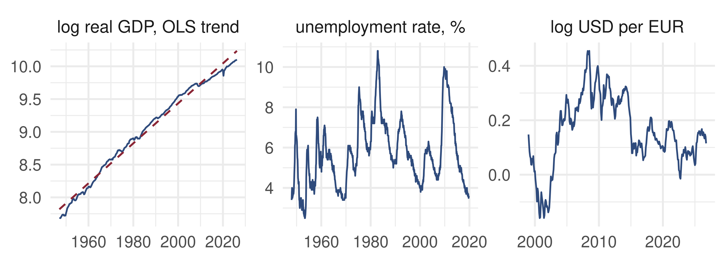
📈 The question

1. Does log real GDP have a unit root around a linear trend?
2. Does the unemployment rate wander, or return to a natural rate?
3. Is the euro–dollar rate a random walk?

📊 The data

Series: FRED GDPC1 (quarterly, 1947–2026, logs, constant + trend); UNRATE (monthly, 1948–2019, constant); DEXUSEU (daily, 1999–2026, monthly averages, logs, constant)

Test: ADF, lag \(p\) by BIC (\(p\le12\))

# How the CSVs were obtained (not run at render time):
for (id in c("GDPC1", "UNRATE", "DEXUSEU"))
  download.file(paste0("https://fred.stlouisfed.org/graph/fredgraph.csv?id=", id),
                paste0("data/", id, ".csv"))

💰 Case Study: ADF by Hand

rd <- function(f) { d <- read.csv(f); d[[2]] <- suppressWarnings(as.numeric(d[[2]]))
  d <- na.omit(d); d$date <- as.Date(d$observation_date); d }
gdp <- rd("data/GDPC1.csv"); un <- rd("data/UNRATE.csv"); eu <- rd("data/DEXUSEU.csv")
eum <- aggregate(eu$DEXUSEU, list(m = format(eu$date, "%Y-%m")), mean)
adf <- function(x, det, pmax = 12) {
  dx <- diff(x); fitp <- function(p, i) {
    X <- cbind(x[i - 1], 1); if (det == "trend") X <- cbind(X, i)
    if (p > 0) for (j in 1:p) X <- cbind(X, dx[i - 1 - j])
    f <- lm.fit(X, x[i]); s2 <- sum(f$residuals^2) / (length(i) - ncol(X))
    list(f = f, k = ncol(X), se = sqrt(s2 * solve(crossprod(X))[1, 1])) }
  i0 <- (pmax + 2):length(x)
  bic <- sapply(0:pmax, function(p) { r <- fitp(p, i0)
    length(i0) * log(mean(r$f$residuals^2)) + r$k * log(length(i0)) })
  p <- which.min(bic) - 1; r <- fitp(p, (p + 2):length(x)); b <- r$f$coefficients[1]
  c(p = p, T = length(x) - p - 1, rho = round(b, 4), tau = round((b - 1) / r$se, 2),
    crit_5pct = if (det == "trend") -3.41 else -2.86)
}
rbind(log_GDP = adf(log(gdp$GDPC1), "trend"), unemployment = adf(un$UNRATE, "const"),
      log_EURUSD = adf(log(eum$x), "const"))

             p   T    rho   tau crit_5pct
log_GDP      0 317 0.9899 -1.25     -3.41
unemployment 5 858 0.9830 -4.17     -2.86
log_EURUSD   1 332 0.9819 -2.08     -2.86

Read the tau column against crit_5pct: reject the unit root only when tau is further left.

💰 Case Study: What the Data Say

What the data say: log GDP (\(\tau=-1.25\)) and the euro (\(\tau=-2.08\)) do not reject the unit root: GDP stayed below its pre-2008 trend. Unemployment rejects (\(\tau=-4.17\)): very persistent, yet mean-reverting. A non-rejection is equally consistent with \(\rho=0.99\).

📝 Quiz #1: Critical Values

A DF regression with a constant (no trend) gives \(\tau=-2.40\). At the 5% level you should:

• Not reject the unit root, since \(-2.40>-2.86\)
• Reject the unit root, since \(-2.40<-1.645\)
• Reject the unit root, since \(|-2.40|>1.96\)
• Not reject, since \(\tau\) must be positive to reject

📝 Quiz #2: Why ADF Adds Lags

In the augmented DF regression \(x_t=\rho x_{t-1}+\sum_{j=1}^p\alpha_j\Delta x_{t-j}+\varepsilon_t\), what is the role of the lagged differences?

• They absorb the serial correlation in \(\Delta x_t\), so that \(\varepsilon_t\) is serially uncorrelated and the DF tables apply
• They remove the deterministic trend
• They make \(x_t\) stationary under the null
• They raise the power against \(\rho=0.999\)

📝 Quiz #3: Pivotal

Why can the DF distribution be tabulated once and for all, while the stationary limit \(N(0,1-\rho^2)\) cannot?

• The DF limit contains no unknown parameter; the stationary one depends on \(\rho\)
• The DF limit is normal
• The DF limit does not depend on the deterministic terms
• The stationary limit has infinite variance

📋 Key Formulas

DF coefficient	\(T(\hat\rho-1)\xrightarrow{d}\int_0^1\mathcal B\,d\mathcal B\big/\int_0^1\mathcal B^2dr\)
DF \(t\)-ratio	\(\tau\xrightarrow{d}\int_0^1\mathcal B\,d\mathcal B\big/\big(\int_0^1\mathcal B^2dr\big)^{1/2}\)
constant / trend	replace \(\mathcal B\) by \(\bar{\mathcal B}=\mathcal B-\int\mathcal B\), or \(\tilde{\mathcal B}=\mathcal B-b_0-b_1r\)
5% points, \(\tau\)	\(-1.94\), \(-2.86\), \(-3.41\)
correlated errors	limit gains \(+\lambda/\omega^2\) in the numerator, \(\lambda=\sum_{j\ge1}\Gamma_j\)
Phillips–Perron	\(Z=T(\hat\rho-1)-\hat\lambda\big/\big(T^{-2}\sum x_{t-1}^2\big)\)
ADF	\(T(\hat\rho-1)/(1-\sum_j\hat\alpha_j)\), \(p\) by BIC

📋 Summary

• Under a unit root \(\hat\rho\) converges at rate \(T\) to a pivotal, left-skewed DF distribution
• The test is left-tailed; the critical values come from DF tables, never from \(N(0,1)\)
• Always include a constant; include a trend for trending series
• Serial correlation adds a nuisance term: remove it with Phillips–Perron or with ADF lags
• A unit root and \(\rho=0.999\) are indistinguishable in a sample and differ only in the long run

📚 Further Reading

• Hamilton, J. D. (1994), Time Series Analysis, ch. 17
• Tsay, R. S. (2010), Analysis of Financial Time Series, §2.7
• Dickey, D. A. and Fuller, W. A. (1979), JASA; Said, S. E. and Dickey, D. A. (1984), Biometrika
• Phillips, P. C. B. and Perron, P. (1988), Biometrika
• MacKinnon, J. G. (1996), Journal of Applied Econometrics (critical values)
• Schwert, G. W. (1989), JBES (size of the tests with MA errors)

Next lecture: Nonlinear Models and Threshold Autoregression. A series can be very persistent without a unit root, and white noise can still be predictable.

⬅ Previous lecture: 09 · Trends, Unit Roots and Brownian Motion