Time Series Econometrics

Lecture 11: Nonlinear Models and Threshold Autoregression

Samir Orujov, PhD

Open lecture notes, after Stanislav Anatolyev’s course (2016)

🎬 The Idea in 3 Minutes

⬅ Previous lecture: 10 · Dickey–Fuller, Phillips–Perron and ADF Tests

A short film with the intuition. Watch it before the slides, or after. Captions: CC button.

🎯 Learning Objectives

By the end of this lecture, you will be able to:

• Explain two reasons to leave linear models: persistence without a unit root, and predictable white noise

• Write down a threshold autoregression and choose its threshold variable for a given series

• Judge stationarity of a TAR, including one with an explosive regime

• Estimate a SETAR by concentrated least squares over a trimmed grid

• State the asymptotic behaviour of \(\hat\gamma\) and of the slope estimates

🔁 Warm-up from last time

Lecture 10: \(T=300\) observations from \(x_t=0.999\,x_{t-1}+\varepsilon_t\). How often does a 5% DF test (with a constant) reject the unit root?

• About 5% of the time
• About 95% of the time
• About 50% of the time
• Never, since the series is stationary

🗺️ Where We Are

Lecture 10 ended on a limitation: in a sample, a unit root and a root of \(0.999\) look the same. A unit-root test measures persistence, nothing more.

Some series are persistent, yet economic theory says they must revert: the real exchange rate under purchasing power parity is the standard case. A linear AR can only make such a series uniformly persistent. Today the dynamics are allowed to depend on the state of the series.

❓ The Question

Does unemployment rise faster than it falls?

In US recessions the unemployment rate jumps by several points within a year. In expansions it drifts down by a tenth of a point a month for years.

A linear AR for \(\Delta u_t\) has one set of coefficients, so a rise and a fall of the same size must be followed by mirror-image paths. If the dynamics differ between “unemployment rising” and “unemployment falling”, a linear model averages two different economies into one that exists in neither.

💡 Persistence Without a Unit Root

Nonlinear modelling can build a bridge between empirical properties and economic theory.

• Empirically, real exchange rates are very persistent; unit-root tests often fail to reject.
• In theory, PPP says the real exchange rate fluctuates around zero (its log deviation from parity).
• A nonlinear model reconciles the two: little or no reversion near parity, strong reversion far from it.

The series is persistent, but it has no unit root. We return to this example with numbers below.

💡 Predictable White Noise

Let \(\varepsilon_t\) be strong white noise (i.i.d., mean 0, variance 1) and \[y_t=\varepsilon_t+\theta\,\varepsilon_{t-1}\varepsilon_{t-2}.\]

For \(j\neq0\), every term of \(E(y_ty_{t-j})\) contains a factor \(\varepsilon_s\) that appears exactly once, so it vanishes: \(\operatorname{cov}(y_t,y_{t-j})=0\). Thus \(y_t\) is white noise, though not independent.

The best linear forecast is therefore \(\hat y^{\,\text{lin}}_{t+1}=0\). The conditional mean is not: \[\hat y^{\,\text{nonlin}}_{t+1}=E(y_{t+1}\mid\mathcal F_t)=\theta\,\varepsilon_t\varepsilon_{t-1}.\] A nonlinear model can reveal information that no linear model can detect.

💻 White Noise You Can Forecast

n <- 5000; theta <- 0.8; e <- rnorm(n + 2)
y  <- e[3:(n + 2)] + theta * e[2:(n + 1)] * e[1:n]
round(acf(y, lag.max = 5, plot = FALSE)$acf[2:6], 3)     # autocorrelations, lags 1-5
f_nonlin <- theta * e[2:(n + 1)] * e[1:n]                # E(y_t | past)
c(R2_linear    = 0,
  R2_nonlinear = round(1 - mean((y - f_nonlin)^2) / var(y), 3),
  theory       = round(theta^2 / (1 + theta^2), 3))

[1] -0.011 -0.008 -0.001 -0.018 -0.012
   R2_linear R2_nonlinear       theory 
       0.000        0.372        0.390 

Every autocorrelation is within \(\pm0.02\) of zero, yet the conditional mean explains over a third of the variance. A close relative is the bilinear model: an ARMA plus cross terms \(\sum_{i,j}\psi_{ij}x_{t-i}\varepsilon_{t-j}\).

📐 Threshold Autoregression (TAR)

Models with regimes are the nonlinear family most used in economics. In a TAR there are most often two regimes, with linear AR dynamics in each: \[x_t=\begin{cases}\mu_1+\rho_1x_{t-1} & \text{if } q_{t-1}\le\gamma\\[2pt] \mu_2+\rho_2x_{t-1} & \text{if } q_{t-1}>\gamma\end{cases}\;+\;\varepsilon_t, \qquad E_{t-1}\varepsilon_t=0,\ \operatorname{var}_{t-1}\varepsilon_t=\sigma^2.\]

• The switch is driven by an event: the threshold variable \(q_{t-1}\) exceeds the threshold \(\gamma\).
• \(q_{t-1}\) must be realised in the previous period, so the regime is known before \(x_t\) is drawn.
• The switches are endogenous when \(q_{t-1}\) depends on the series itself.

📐 SETAR, and Choosing \(q_{t-1}\)

If \(q_{t-1}=x_{t-d}\) for a known or unknown delay \(d\), the model is a self-exciting TAR (SETAR). The choice of \(q_{t-1}\) depends on the frequency and nature of the data:

Series	Threshold variable	Regimes
GNP growth, quarterly	\(q_{t-1}=y_{t-2}\)	contraction / expansion
unemployment, monthly	\(q_{t-1}=\Delta x_{t-d}\) or \(x_{t-1}-x_{t-d}\)	rising / falling
nominal exchange rate, weekly returns	\(q_{t-1}=\frac15\sum_{j=1}^{5}\lvert x_{t-j}\rvert\)	high / low volatility
real exchange rate, quarterly	\(q_{t-1}=\lvert x_{t-1}\rvert\)	near / far from PPP

📐 The Real Exchange Rate Band

Let \(x_t\) be the log deviation of the real exchange rate from PPP, and \(q_{t-1}=|x_{t-1}|\):

• inner regime, \(|x_{t-1}|\le\gamma\): estimates give \(\rho_1=1.06\), locally explosive;
• outer regime, \(|x_{t-1}|>\gamma\): \(\rho_2\approx0.92\), mean-reverting.

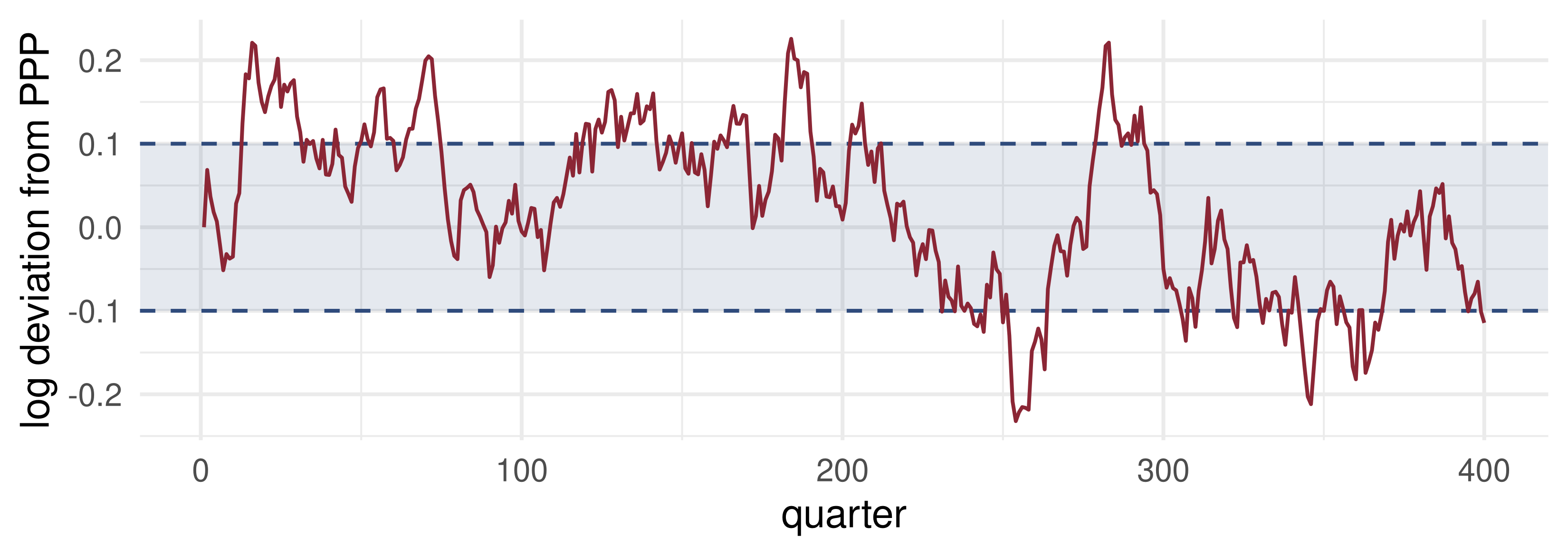
Inside the band, transaction costs make arbitrage unprofitable, and the rate drifts away from parity. Outside it, arbitrage pulls it back. A unit-root test will typically find \(I(1)\), yet the outer regime forces the process back towards the band: it is globally stationary.

💻 Simulating the Band

Explosive inside the shaded band, \(\rho_1=1.06\); mean-reverting outside it, \(\rho_2=0.92\); \(\gamma=0.10\), \(\sigma=0.03\).

💻 The Band Fools the DF Test

dft <- function(x) { y <- x[-1]; X <- cbind(1, x[-length(x)]); f <- lm.fit(X, y)
  s2 <- sum(f$residuals^2) / (length(y) - 2)
  (f$coefficients[2] - 1) / sqrt(s2 * solve(crossprod(X))[2, 2]) }
c(rejection_rate_5pct = mean(replicate(2000, dft(sim_band(160)) < -2.86)))

rejection_rate_5pct 
             0.2065 

The process is globally stationary, yet in forty years of quarterly data the DF test fails to reject the unit root about four times in five.

📐 Stationarity of a TAR

\(|\rho_1|<1\) and \(|\rho_2|<1\) is sufficient but not necessary.

• One regime may have a unit root, or even \(\rho>1\), and the process can still be globally stationary.
• What makes this possible is an endogenous switch: the threshold variable depends on \(x\) itself, so an explosive regime pushes the process out of that regime.

For SETAR(1) with \(q_{t-1}=x_{t-1}\) and zero intercepts, the process is ergodic if and only if \[\rho_1<1,\qquad \rho_2<1,\qquad \rho_1\rho_2<1\] (Petrucelli and Woolford, 1984). So \(\rho_1=-3\), \(\rho_2=0.2\) is stationary: \(|\rho_1|>1\) but \(\rho_1\rho_2=-0.6<1\).

🔧 Extensions: Lags and Regimes

Different lag orders. Regime \(j\) has its own AR(\(p_j\)): \[x_t=\mu_j+\rho_{j,1}x_{t-1}+\dots+\rho_{j,p_j}x_{t-p_j}+\varepsilon_t\quad\text{in regime } j .\] Choose \((p_1,p_2)\) by minimising \(IC_1+IC_2\), for example \[BIC_j=T_j\log\hat\sigma_j^2+p_j\log T_j,\] where \(T_j\) is the number of observations in regime \(j\).

Multiple regimes, same threshold variable, with \(\gamma_0<\gamma_1<\dots<\gamma_m\): \[x_t=\mu_j+\rho_jx_{t-1}+\varepsilon_t\quad\text{if }\gamma_{j-1}\le q_{t-1}<\gamma_j,\qquad j=1,\dots,m.\]

🔧 Extensions: Two Thresholds

Four regimes, governed by \(x_{t-1}\) and \(x_{t-2}\) with thresholds \(\gamma_1,\gamma_2\): \[x_t=\begin{cases}\mu_1+\rho_1x_{t-1} & \text{if }x_{t-2}\le\gamma_2,\ x_{t-1}\le\gamma_1\\ \mu_2+\rho_2x_{t-1} & \text{if }x_{t-2}\le\gamma_2,\ x_{t-1}>\gamma_1\\ \mu_3+\rho_3x_{t-1} & \text{if }x_{t-2}>\gamma_2,\ x_{t-1}\le\gamma_1\\ \mu_4+\rho_4x_{t-1} & \text{if }x_{t-2}>\gamma_2,\ x_{t-1}>\gamma_1\end{cases}\;+\;\varepsilon_t .\]

Each added threshold multiplies the number of regimes, and divides the observations available to each.

🔧 Extensions: Rules and Variances

A general switching rule. Replace \(q_{t-1}\lessgtr\gamma\) by a condition on \[f(x_{t-1},\dots,x_{t-d},\vartheta),\] where the form of \(f\) is known a priori, the delay \(d\) may be unknown, and \(\vartheta\) is an unknown finite-dimensional parameter.

Regime-wise heteroskedasticity: \[\operatorname{var}_{t-1}\varepsilon_t=\begin{cases}\sigma_1^2 & \text{if }q_{t-1}\le\gamma\\ \sigma_2^2 & \text{if }q_{t-1}>\gamma\end{cases}\]

Conditional heteroskedasticity: \(\operatorname{var}_{t-1}\varepsilon_t\) not constant, for example GARCH-type errors (Lecture 15).

📐 Estimation: The Problem

Back to the basic model, written with indicators: \[x_t=(\mu_1+\rho_1x_{t-1})\,\mathbb 1\{q_{t-1}\le\gamma\}+(\mu_2+\rho_2x_{t-1})\,\mathbb 1\{q_{t-1}>\gamma\}+\varepsilon_t .\] Parameters: \(\theta=(\mu_1,\rho_1,\mu_2,\rho_2,\gamma,d)\), with \(d\) possibly, and \(\sigma^2\). Because \(\gamma\) is unknown, the model is nonlinear.

Gaussian QML is equivalent to NLLS: \[\min_\theta\sum_t\Big(x_t-(\mu_1+\rho_1x_{t-1})\mathbb 1\{q_{t-1}\le\gamma\}-(\mu_2+\rho_2x_{t-1})\mathbb 1\{q_{t-1}>\gamma\}\Big)^2 .\] With respect to \(\gamma\) the objective is not only non-differentiable but not even continuous. Gradient methods are useless.

🔧 The Concentration Method

Split the parameters into \(\gamma\) and the rest. For fixed \(\gamma\) the model is linear.

1. Grid. Make a grid \(\Gamma\) for \(\gamma\). If \(q\) is a lag of \(x\), put the grid points at the observed values of \(q_{t-1}\). Trim the lowest and highest 10–15%: too few observations in a regime do not allow its parameters to be estimated.
2. OLS for each \(\gamma\in\Gamma\). Regress \(x_t\) on the regime-split regressors and record \(\hat\sigma^2(\gamma)\).
3. Minimise. \(\hat\gamma=\arg\min_{\gamma\in\Gamma}\hat\sigma^2(\gamma)\), and \(\hat\theta=\hat\theta(\hat\gamma)\), the OLS estimates at \(\hat\gamma\).

If \(d\) is unknown, minimise over the pairs \((d,\gamma)\).

✍️ Worked Example: The Data

Six observations, and a TAR with regime means only: \(x_t=\mu_1\mathbb 1\{q_{t-1}\le\gamma\}+\mu_2\mathbb 1\{q_{t-1}>\gamma\}+\varepsilon_t\).

\(q_{t-1}\)	−1.0	−0.6	−0.2	0.1	0.4	0.9
\(x_t\)	−0.5	−0.7	−0.3	0.6	0.4	0.8

Grid. Put candidate thresholds at the observed \(q\). Require at least two observations in each regime: this trims \(\gamma=-1.0\), \(0.4\) and \(0.9\), leaving \[\Gamma=\{-0.6,\ -0.2,\ 0.1\}.\] For each \(\gamma\) the OLS estimates are the two regime means, and \(SSR(\gamma)\) is the sum of squared deviations within regimes.

✍️ Worked Example: The Grid

\(\gamma\)	regime 1	\(\hat\mu_1\)	regime 2	\(\hat\mu_2\)	\(SSR(\gamma)\)
−0.6	−0.5, −0.7	−0.600	−0.3, 0.6, 0.4, 0.8	0.375	0.020 + 0.688 = 0.708
−0.2	−0.5, −0.7, −0.3	−0.500	0.6, 0.4, 0.8	0.600	0.080 + 0.080 = 0.160
0.1	−0.5, −0.7, −0.3, 0.6	−0.225	0.4, 0.8	0.600	0.988 + 0.080 = 1.068

So \(\hat\gamma=-0.2\), \(\hat\mu_1=-0.5\), \(\hat\mu_2=0.6\), \(\hat\sigma^2=0.160/6=0.027\).

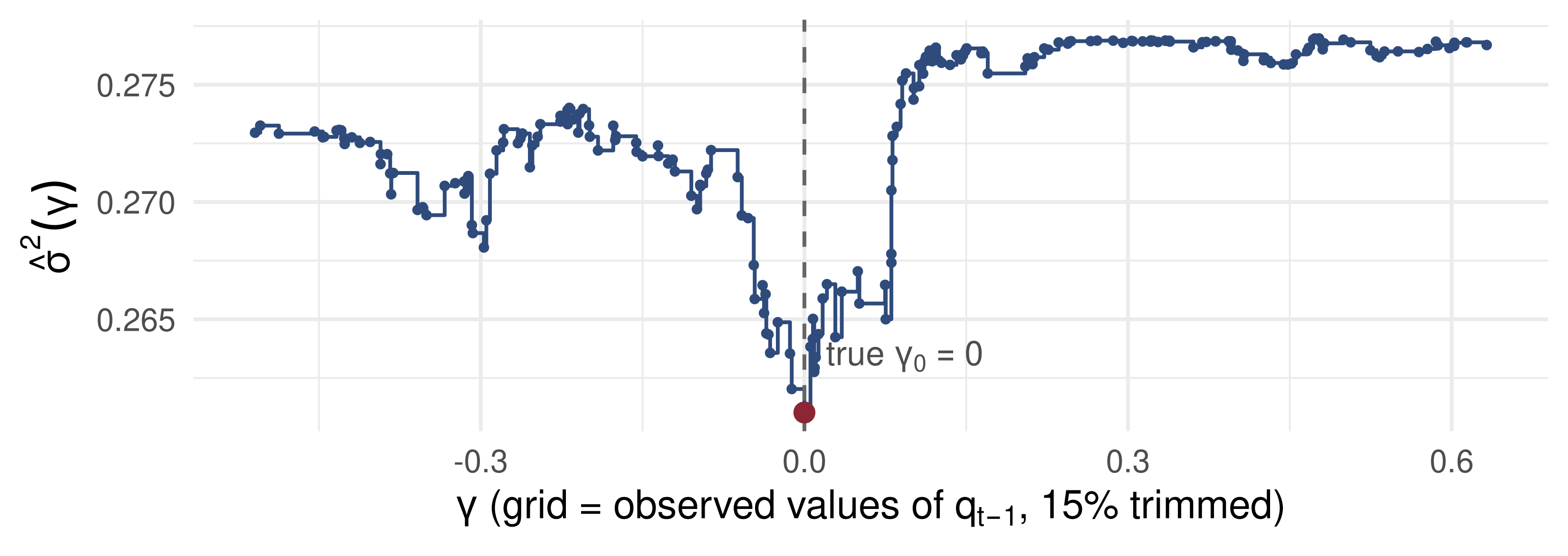
Any \(\gamma\in[-0.2,\,0.1)\) splits the sample identically, so \(\hat\sigma^2(\gamma)\) is flat there: the objective is a step function, and only its values at the observed \(q\) matter.

💻 SETAR by Hand

set.seed(2028); n <- 300; x <- numeric(n + 1)
for (t in 2:(n + 1)) x[t] <- if (x[t - 1] <= 0) 0.4 + 0.6 * x[t - 1] + 0.5 * rnorm(1) else
                                               -0.2 + 0.3 * x[t - 1] + 0.5 * rnorm(1)
y <- x[-1]; q <- x[-(n + 1)]                          # q_{t-1} = x_{t-1}: self-exciting
setar_s2 <- function(g) { I <- q <= g; J <- !I              # regime indicators
  mean(lm.fit(cbind(I, I * q, J, J * q), y)$residuals^2) }
grid <- sort(q); grid <- grid[grid >= quantile(q, 0.15) & grid <= quantile(q, 0.85)]
s2   <- sapply(grid, setar_s2)
g_hat <- grid[which.min(s2)]; I <- q <= g_hat; J <- !I
b <- lm.fit(cbind(I, I * q, J, J * q), y)$coefficients
round(c(gamma_hat = g_hat, mu1 = b[[1]], rho1 = b[[2]], mu2 = b[[3]], rho2 = b[[4]],
        grid_points = length(grid)), 3)

  gamma_hat         mu1        rho1         mu2        rho2 grid_points 
      0.000       0.311       0.485      -0.122       0.296     210.000 

True values: \(\gamma_0=0\), \((\mu_1,\rho_1)=(0.4,0.6)\), \((\mu_2,\rho_2)=(-0.2,0.3)\). The threshold is found almost exactly; the slopes carry ordinary sampling error of about \(\pm0.1\).

📊 The Objective Is a Step Function

Flat between neighbouring observations, jumping at each one; rough overall, with a sharp dip whose lowest step (red) is \(\hat\gamma\).

📐 Asymptotic Theory

Because of the discontinuity, the usual asymptotic theory does not apply. Yet the outcome is good news.

• \(\hat\mu_1,\hat\rho_1,\hat\mu_2,\hat\rho_2,\hat\sigma^2\) are standard: consistent, \(\sqrt T\)-rate, asymptotically normal, with the same limit as if \(\gamma\) were known.
• \(\hat\gamma\) is \(T\)-consistent: \(\hat\gamma-\gamma=O_p(T^{-1})\). Because it converges so fast, we may act as if \(\hat\gamma\) were the true value when doing inference on the slopes.
• The discontinuity looks like a curse; it is in fact a blessing.

The catch: the limit of \(T(\hat\gamma-\gamma)\) is non-pivotal. It depends on unknown parameters and is very hard to standardise. How, then, do we build a confidence interval for \(\gamma\)? That question opens the next lecture.

🧠 Think–Pair–Share

1. In the step plot, why is \(\hat\sigma^2(\gamma)\) constant between two neighbouring observed values of \(q_{t-1}\)?
2. What goes wrong if we search \(\gamma\) all the way to the smallest observed \(q_{t-1}\)?
3. A colleague estimates \(\gamma\) with a Newton–Raphson routine started at the median of \(q_{t-1}\). What will happen?

✅ Think–Pair–Share: Solution

1. \(\hat\sigma^2(\gamma)\) depends on \(\gamma\) only through the split \(\{t: q_{t-1}\le\gamma\}\). Between two neighbouring observations the split does not change, so neither does the OLS fit.

2. Regime 1 would hold one or two observations: its two parameters are barely or not at all estimable, and \(\hat\sigma^2(\gamma)\) can be driven down by fitting a handful of points exactly. Trimming 10–15% at each end prevents this.

3. The derivative of a step function is zero wherever it exists. Newton–Raphson sees a flat objective and stops where it started. Grid search over observed values is exact, and cheap: one OLS per grid point.

💰 Case Study: Unemployment Regimes

📈 The question

1. Do the dynamics of \(\Delta u_t\) change when unemployment is above its level a year earlier?
2. Where is the threshold?
3. How different are the two regimes?

📊 The data

Series: US unemployment rate, FRED UNRATE, monthly, Jan 1948 – Dec 2019

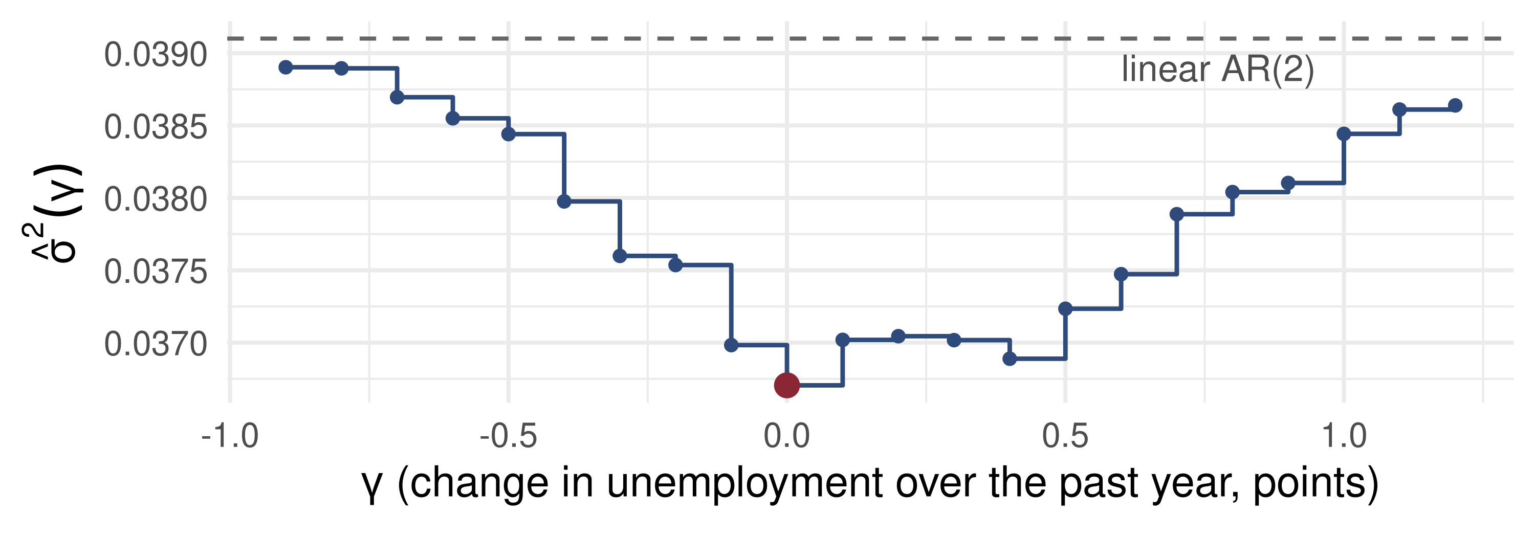
\(x_t=\Delta u_t\), two lags in each regime; \(q_{t-1}=u_{t-1}-u_{t-13}\), the change over the past year; grid trimmed 15%

2020 is left out: one month’s jump of 10 points would dominate least squares

download.file("https://fred.stlouisfed.org/graph/fredgraph.csv?id=UNRATE",
              "data/UNRATE.csv")   # then keep Jan 1948 - Dec 2019

💰 Case Study: The Estimates

un <- read.csv("data/UNRATE.csv"); u <- un$UNRATE; N <- length(u)
du <- c(NA, diff(u)); tt <- 14:N                    # d = 12 needs u_{t-13}
yy <- du[tt]; Z <- cbind(1, du[tt - 1], du[tt - 2])
qq <- round(u[tt - 1] - u[tt - 13], 1)              # one-decimal data: avoid float noise
G  <- sort(unique(qq)); G <- G[G >= quantile(qq, 0.15) & G <= quantile(qq, 0.85)]
s2_u <- sapply(G, function(g) { I <- qq <= g
  mean(lm.fit(cbind(Z * I, Z * !I), yy)$residuals^2) })
gh <- G[which.min(s2_u)]; I <- qq <= gh
fit <- lm(yy ~ 0 + cbind(Z * I, Z * !I)); b <- coef(fit); se <- sqrt(diag(vcov(fit)))
print(c(T = length(yy), grid_from = min(G), grid_to = max(G), gamma_hat = gh,
        share_falling = round(mean(I), 2)))
round(cbind(falling = b[1:3], se = se[1:3], rising = b[4:6], se = se[4:6]), 3) |>
  `rownames<-`(c("const", "du(t-1)", "du(t-2)"))

            T     grid_from       grid_to     gamma_hat share_falling 
       851.00         -0.90          1.20          0.00          0.67 
        falling    se rising    se
const    -0.041 0.009  0.018 0.013
du(t-1)  -0.149 0.052  0.138 0.045
du(t-2)   0.035 0.051  0.367 0.046

Read the columns side by side: a steady fall with no momentum against a rise that feeds on itself.

💰 Case Study: What the Data Say

What the data say: \(\hat\gamma=0\). When unemployment is no higher than a year ago it drifts down by about 0.04 points a month; when it is higher, it rises with momentum (coefficient 0.37 on \(\Delta u_{t-2}\)). The model is silent on whether the gain over the linear AR(2) is more than chance: next lecture.

📝 Quiz #1: The Threshold Variable

Which threshold variable separates high- and low-volatility regimes for weekly exchange-rate returns \(x_t\)?

• \(q_{t-1}=\frac15\sum_{j=1}^5|x_{t-j}|\)
• \(q_{t-1}=x_{t-1}\)
• \(q_{t-1}=x_t\)
• \(q_{t-1}=\frac15\sum_{j=1}^5x_{t-j}\)

📝 Quiz #2: Stationarity

A SETAR(1) with \(q_{t-1}=x_{t-1}\) and zero intercepts has \(\rho_1=1.2\) in the lower regime and \(\rho_2=0.5\) in the upper. Is it stationary?

• No: the condition \(\rho_1<1\) fails
• Yes: \(\rho_1\rho_2=0.6<1\)
• Yes: the upper regime pulls it back
• Only if \(\sigma^2\) is small

📝 Quiz #3: Superconsistency

\(\hat\gamma\) is \(T\)-consistent. What does this buy us?

• Inference on \(\mu_j,\rho_j\) can proceed as if \(\gamma\) were known
• A normal confidence interval \(\hat\gamma\pm1.96\,SE(\hat\gamma)\)
• The objective becomes differentiable in large samples
• No trimming is needed

📋 Key Formulas

predictable white noise	\(y_t=\varepsilon_t+\theta\varepsilon_{t-1}\varepsilon_{t-2}\), \(E(y_{t+1}\mid\mathcal F_t)=\theta\varepsilon_t\varepsilon_{t-1}\)
TAR	\(x_t=(\mu_1+\rho_1x_{t-1})\mathbb 1\{q_{t-1}\le\gamma\}+(\mu_2+\rho_2x_{t-1})\mathbb 1\{q_{t-1}>\gamma\}+\varepsilon_t\)
SETAR	\(q_{t-1}=x_{t-d}\)
SETAR(1) ergodic	\(\rho_1<1,\ \rho_2<1,\ \rho_1\rho_2<1\)
lag orders	\(\min_{p_1,p_2}(IC_1+IC_2)\), \(BIC_j=T_j\log\hat\sigma_j^2+p_j\log T_j\)
concentration	\(\hat\gamma=\arg\min_{\gamma\in\Gamma}\hat\sigma^2(\gamma)\), \(\hat\theta=\hat\theta(\hat\gamma)\)
rates	\(\hat\gamma-\gamma=O_p(T^{-1})\); slopes \(\sqrt T\)-normal

📋 Summary

• Nonlinear models give persistence without a unit root, and forecasts where linear ones see white noise
• A TAR switches between linear regimes when an observed \(q_{t-1}\) crosses \(\gamma\)
• An endogenous switch can make a TAR stationary despite an explosive regime
• Estimation: OLS for each \(\gamma\) on a trimmed grid of observed values; take the minimum
• Slopes are \(\sqrt T\)-normal as if \(\gamma\) were known; \(\hat\gamma\) is \(T\)-consistent with a non-pivotal limit

📚 Further Reading

• Franses, P. H. and van Dijk, D. (2000), Non-linear Time Series Models in Empirical Finance, ch. 3
• Tsay, R. S. (2010), Analysis of Financial Time Series, ch. 4
• Tong, H. (1990), Non-linear Time Series: A Dynamical System Approach
• Granger, C. W. J. and Andersen, A. P. (1978), An Introduction to Bilinear Time Series Models
• Chan, K. S. (1993), Annals of Statistics (consistency of \(\hat\gamma\))
• Petrucelli, J. and Woolford, S. (1984), J. Applied Probability; Hansen, B. E. (1997), Studies in Nonlinear Dynamics and Econometrics

Next lecture: Threshold Inference and Smooth Transition. A confidence set for \(\gamma\), a test of linearity, and regimes that blend.

⬅ Previous lecture: 10 · Dickey–Fuller, Phillips–Perron and ADF Tests