Time Series Econometrics

Lecture 12: Threshold Inference and Smooth Transition

Samir Orujov, PhD

Open lecture notes, after Stanislav Anatolyev’s course (2016)

🎬 The Idea in 3 Minutes

⬅ Previous lecture: 11 · Nonlinear Models and Threshold Autoregression

A short film with the intuition. Watch it before the slides, or after. Captions: CC button.

🎯 Learning Objectives

By the end of this lecture, you will be able to:

• State Hansen’s likelihood-ratio result for the threshold, and compute its critical values

• Construct a confidence set for \(\gamma\) by inverting \(LR(\gamma)\), and read an asymmetric or disjoint one

• Explain why linearity tests are non-standard when \(\gamma\) is unidentified, and run a sup-F test with the fixed-regressor bootstrap

• Write down LSTAR and ESTAR models, and describe their limits as \(\delta\to0\) and \(\delta\to\infty\)

🔁 Warm-up from last time

Lecture 11: in concentrated least squares for a TAR, what does \(\hat\sigma^2(\gamma)\) look like as a function of \(\gamma\)?

• A step function, constant between neighbouring observed values of \(q_{t-1}\)
• A smooth parabola with its minimum at \(\hat\gamma\)
• A straight line
• A continuous function with a kink at \(\hat\gamma\)

🗺️ Where We Are

Lecture 11 ended with good news and an open question. The slopes of a TAR are \(\sqrt T\)-normal as if \(\gamma\) were known, and \(\hat\gamma\) is \(T\)-consistent. But the limit of \(T(\hat\gamma-\gamma)\) is non-pivotal.

Today: how to build a confidence set for \(\gamma\) anyway; how to test whether there is a threshold at all; and what happens when the switch between regimes is gradual rather than abrupt.

❓ The Question

Three questions about unemployment

Lecture 11 found that US unemployment dynamics switch when unemployment is above its level of a year earlier, with \(\hat\gamma=0\).

1. How precisely is the threshold located? Could it be \(0.3\) points instead of \(0\)?
2. Is the gain over a linear AR(2) real, or the product of searching over 22 candidate thresholds?
3. Do the regimes switch like a light, or fade into each other like a dimmer?

📐 Recap: TAR and Its Estimator

\[x_t=\begin{cases}\mu_1+\rho_1x_{t-1} & \text{if } q_{t-1}\le\gamma_0\\ \mu_2+\rho_2x_{t-1} & \text{if } q_{t-1}>\gamma_0\end{cases}\;+\;\varepsilon_t,\qquad E_{t-1}\varepsilon_t=0,\ \operatorname{var}_{t-1}\varepsilon_t=\sigma^2 .\]

NLLS with concentration gives \(\hat\theta=(\hat\mu_1,\hat\rho_1,\hat\mu_2,\hat\rho_2,\hat\gamma,\hat d)\) and \(\hat\sigma^2\); the integer delay \(d\) is searched jointly with \(\gamma\) when unknown.

• \(\hat\gamma\) is superconsistent (\(T\)-consistent), with a non-standard, non-pivotal limit.
• \(\hat\mu_1,\hat\rho_1,\hat\mu_2,\hat\rho_2,\hat\sigma^2\) are \(\sqrt T\)-consistent and asymptotically normal: we can act as though \(\hat\gamma=\gamma_0\).

📐 Hansen’s Result

Define, with \(\hat\sigma^2=\hat\sigma^2(\hat\gamma)=\min_\gamma\hat\sigma^2(\gamma)\), \[LR(\gamma)=T\,\frac{\hat\sigma^2(\gamma)-\hat\sigma^2}{\hat\sigma^2}.\]

Theorem (Hansen, 2000)

If the threshold effect shrinks, but slowly, \((\mu_1-\mu_2,\,\rho_1-\rho_2)'\to0\) while \(\sqrt T(\mu_1-\mu_2,\,\rho_1-\rho_2)'\to\infty\), then under conditional homoskedasticity \[LR(\gamma_0)\ \xrightarrow{d}\ \xi=\max_{r\in\mathbb R}\{2B(r)-|r|\}.\]

\(B\) is a two-sided standard Brownian motion on \(\mathbb R\) with \(B(0)=0\): two independent Brownian motions glued at the origin.

📐 The Limit Is Pivotal

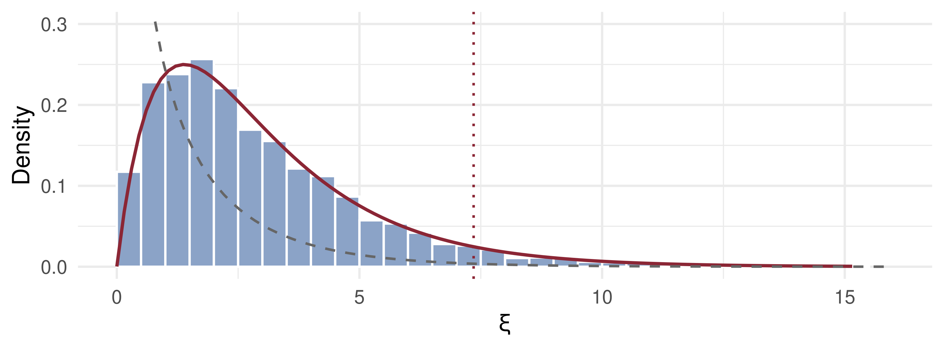
\(\xi\) is a random variable, and its distribution is known in closed form: \[\Pr\{\xi\le u\}=\left(1-e^{-u/2}\right)^2,\qquad u\ge0 .\] It contains no unknown parameter: it is pivotal.

Inverting the CDF at \(1-\alpha\): \[\left(1-e^{-c/2}\right)^2=1-\alpha\ \iff\ e^{-c/2}=1-\sqrt{1-\alpha}\ \iff\ c_{1-\alpha}=-2\ln\!\big(1-\sqrt{1-\alpha}\big).\]

Without conditional homoskedasticity the limit is \(\eta^2\xi\), with a nuisance scale \(\eta^2\) that must be estimated.

✍️ Worked Example: Critical Values

Compute \(c_{1-\alpha}=-2\ln(1-\sqrt{1-\alpha})\) step by step.

\(\alpha\)	\(\sqrt{1-\alpha}\)	\(1-\sqrt{1-\alpha}\)	\(\ln(\cdot)\)	\(c_{1-\alpha}\)
0.10	0.94868	0.05132	−2.9699	5.94
0.05	0.97468	0.02532	−3.6761	7.35
0.01	0.99499	0.00501	−5.2958	10.59

Compare \(\chi^2(1)\): 2.71, 3.84, 6.63. The threshold critical values are roughly twice as large: \(\xi\) is the maximum of a process over the whole line, not one squared normal.

💻 Simulating \(\xi\)

h <- 0.001; R <- 20; m <- R / h; r <- (1:m) * h
xi <- replicate(3000, {
  up <- cumsum(rnorm(m, sd = sqrt(h)))         # B(r), r > 0
  dn <- cumsum(rnorm(m, sd = sqrt(h)))         # B(-r), independent side
  max(0, 2 * up - r, 2 * dn - r) })            # r = 0 gives 0
crit <- function(a) -2 * log(1 - sqrt(1 - a))
rbind(simulated = quantile(xi, c(0.90, 0.95, 0.99)),
      exact     = crit(c(0.10, 0.05, 0.01))) |> round(2)

           90%  95%   99%
simulated 5.83 7.28 10.67
exact     5.94 7.35 10.59

Simulation and formula agree to about 0.1. The grid sees the path only at its nodes, which pulls the simulated values slightly down; Monte Carlo noise does the rest.

📊 The Distribution of \(\xi\)

Bars: simulated \(\xi\). Red: the density \((1-e^{-u/2})e^{-u/2}\). Dashed: \(\chi^2(1)\). Dotted: \(c_{0.95}=7.35\).

📐 Why Shrinking Threshold Effects?

The condition \((\mu_1-\mu_2,\rho_1-\rho_2)\to0\) is an example of alternative asymptotics.

• The regime parameters are fixed in reality. We pretend that, as \(T\to\infty\), they also move closer, but more slowly than \(T^{-1/2}\).
• Under fixed differences, the limit of \(T(\hat\gamma-\gamma_0)\) depends on the whole distribution of the data, and cannot be standardised.
• The shrinking device trades a little realism for a limit that is easy to use.

Compare weak instruments, where letting the first-stage coefficient shrink at rate \(T^{-1/2}\) gives tractable limits.

📐 A Confidence Set by Inversion

Collect the values of \(\gamma\) that the LR statistic does not reject: \[CI_{1-\alpha}(\gamma_0)=\big\{\gamma\in\Gamma:\ LR(\gamma)\le c_{1-\alpha}\big\},\qquad c_{0.95}=7.35 .\]

On a plot of \(LR(\gamma)\): draw a horizontal line at \(c_{1-\alpha}\), and keep the \(\gamma\) where the curve lies below it.

The set is built in a non-standard way, so

• it need not be symmetric around \(\hat\gamma\);
• it may be disjoint: \(LR(\gamma)\) is jagged, and a second dip below the line adds a separate piece.

💻 \(LR(\gamma)\) by Hand

set.seed(2028); n <- 300; x <- numeric(n + 1)
for (t in 2:(n + 1)) x[t] <- if (x[t - 1] <= 0) 0.4 + 0.6 * x[t - 1] + 0.5 * rnorm(1) else
                                               -0.2 + 0.3 * x[t - 1] + 0.5 * rnorm(1)
y <- x[-1]; q <- x[-(n + 1)]
s2_of <- function(g) { I <- q <= g; J <- !I
  mean(lm.fit(cbind(I, I * q, J, J * q), y)$residuals^2) }
grid <- sort(q); grid <- grid[grid >= quantile(q, 0.15) & grid <= quantile(q, 0.85)]
s2 <- sapply(grid, s2_of); g_hat <- grid[which.min(s2)]
LR <- n * (s2 - min(s2)) / min(s2)
inside <- grid[LR <= crit(0.05)]
round(c(gamma_hat = g_hat, ci_low = min(inside), ci_high = max(inside),
        points_in_set = length(inside), grid_points = length(grid)), 3)

    gamma_hat        ci_low       ci_high points_in_set   grid_points 
        0.000        -0.047         0.081        28.000       210.000 

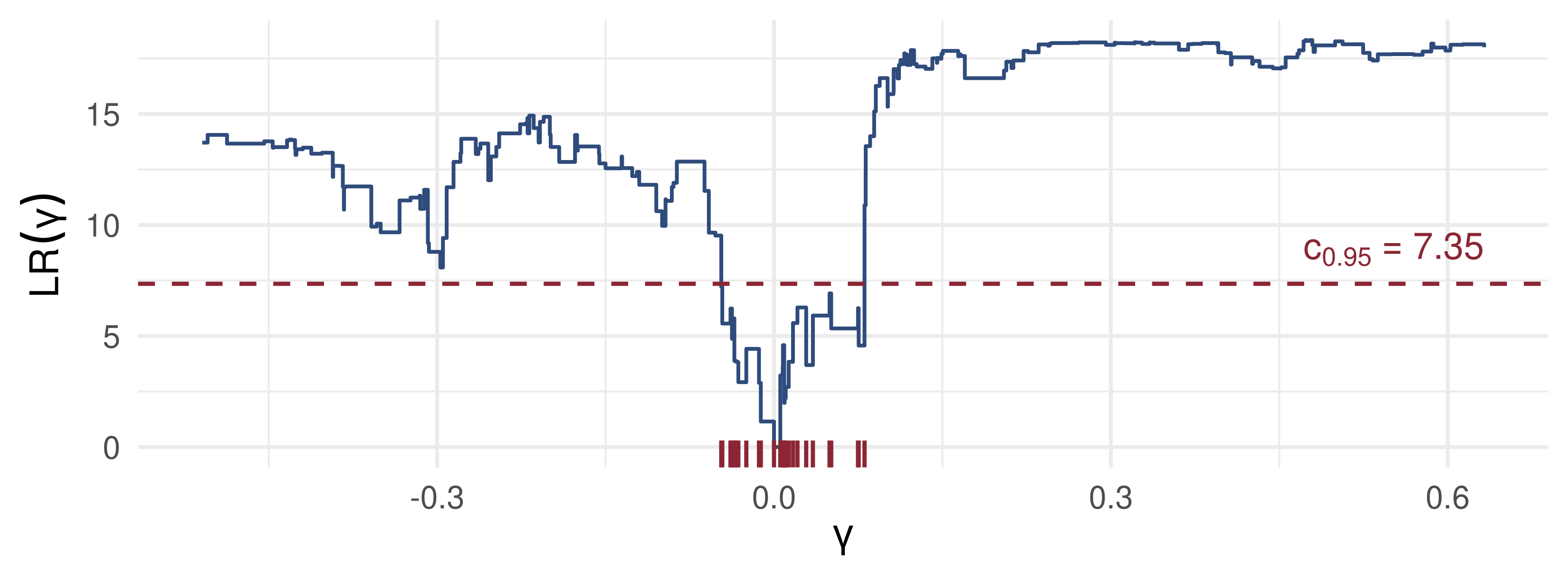
The 95% set runs from about \(-0.05\) to \(0.08\) around \(\hat\gamma\approx0\): it is not centred on \(\hat\gamma\).

📊 Reading the LR Plot

Red ticks on the axis: the grid points with \(LR(\gamma)\le7.35\), the 95% confidence set. Its two sides are not the same length.

📐 Is There a Threshold at All?

\[H_0:\ \mu_1=\mu_2,\ \rho_1=\rho_2\ \text{(linearity)}\qquad H_A:\ \mu_1\neq\mu_2\ \text{or}\ \rho_1\neq\rho_2 .\]

This is testing when a nuisance parameter is not identified under the null. If we impose \(H_0\), the two regimes coincide and \(\gamma_0\) loses its meaning.

Consequently \[W,\ F,\ LR,\ LM\ \ \overset{d}{\underset{H_0}{\not\to}}\ \ \chi^2,\qquad t\ \ \overset{d}{\underset{H_0}{\not\to}}\ \ N(0,1).\] For each fixed \(\gamma\) the usual theory holds; but \(\gamma\) is chosen by searching, and the search inflates the statistic (Davies, 1977, 1987).

📐 The sup-F Statistic

For each \(\gamma\) in the trimmed set \(\Gamma\), compare the linear AR with the TAR at \(\gamma\): \[F(\gamma)=T\,\frac{\tilde\sigma^2-\hat\sigma^2(\gamma)}{\hat\sigma^2(\gamma)},\qquad \sup F=\max_{\gamma\in\Gamma}F(\gamma)=F(\hat\gamma),\] where \(\tilde\sigma^2\) is the residual variance of the linear model. The last equality holds because \(\hat\gamma\) minimises \(\hat\sigma^2(\gamma)\).

Under \(H_0\), \(\sup F\) has a non-standard distribution. Two ways out:

1. alternative asymptotics, or
2. the bootstrap. Bruce Hansen uses a special resampling algorithm, the fixed-regressor bootstrap.

🔧 The Fixed-Regressor Bootstrap

1. Right-hand side: keep \(x_{t-1}\) and \(q_{t-1}\) from the original sample. They are never resampled.
2. Left-hand side: replace \(x_t\) by a draw \(y_t^*\sim\) i.i.d. \(N(0,1)\); under heteroskedasticity, use \(y_t^*=\hat\varepsilon_tz_t\) with \(z_t\sim N(0,1)\).
3. Regress \(y_t^*\) on the fixed regressors, under the null and under the TAR for every \(\gamma\in\Gamma\); compute \(\sup F^*\).
4. Repeat \(B\) times. The p-value is the share of \(\sup F^*\) at or above the sample \(\sup F\).

It works because the null distribution of \(\sup F\) depends on the data only through the regressors; the fixed-regressor bootstrap reproduces exactly that dependence (Hansen, 1996).

💻 What Searching Costs

Fstats <- function(y, xl) { n <- length(y); Z <- cbind(1, xl)
  s2l <- mean(.lm.fit(Z, y)$residuals^2)
  g <- sort(xl); g <- g[g >= quantile(xl, 0.15) & g <= quantile(xl, 0.85)]
  s2u <- sapply(g, function(gg) { I <- xl <= gg; mean(.lm.fit(cbind(Z * I, Z * !I), y)$residuals^2) })
  Fg <- n * (s2l - s2u) / s2u
  c(supF = max(Fg), F_at_median = Fg[ceiling(length(Fg) / 2)]) }
null <- t(replicate(1000, { z <- as.numeric(stats::filter(rnorm(151), 0.5, "recursive"))
  Fstats(z[-1], z[-151]) }))
qs <- apply(null, 2, quantile, c(0.90, 0.95, 0.99))
round(cbind(qs, chisq_2 = qchisq(c(0.90, 0.95, 0.99), df = 2)), 2)

     supF F_at_median chisq_2
90%  9.97        4.53    4.61
95% 11.74        5.62    5.99
99% 15.48        9.16    9.21

At a fixed \(\gamma\), \(F\) behaves like \(\chi^2(2)\). Taking the maximum roughly doubles the 95% point.

🧠 Think–Pair–Share

1. A TAR gives \(\sup F=9.5\). A colleague compares it with \(\chi^2(2)\), whose 99% point is 9.21, and declares a threshold at 1%. What is wrong?
2. A 95% confidence set for \(\gamma\) is \([-0.1,\,0.1]\cup[0.3,\,0.4]\). Is this a mistake?
3. Why does the fixed-regressor bootstrap not simulate a whole new AR path for \(x_t^*\)?

✅ Think–Pair–Share: Solution

1. \(\sup F\) is a maximum over many correlated \(F(\gamma)\). Under \(H_0\) its 95% point is near 12, not 6, so \(9.5\) is not significant even at 10%. The \(\chi^2\) table is for one \(\gamma\) fixed in advance.

2. No. The set is \(\{\gamma:LR(\gamma)\le7.35\}\), and a jagged \(LR(\gamma)\) can dip below the line twice: two locations fit about equally well.

3. Under \(H_0\) the distribution of \(\sup F\) depends on the data only through the regressors. Holding them fixed and redrawing only the error reproduces it, without needing a correct model for the whole path of \(x_t\).

📐 Smooth Transition (STAR)

Replace the indicator by a transition function \(G\) with values in \([0,1]\): \[x_t=(\mu_1+\rho_1x_{t-1})\big(1-G(q_{t-1},\gamma_0,\delta)\big)+(\mu_2+\rho_2x_{t-1})\,G(q_{t-1},\gamma_0,\delta)+\varepsilon_t ,\] with \(E_{t-1}\varepsilon_t=0\), \(\operatorname{var}_{t-1}\varepsilon_t=\sigma^2\). \(\delta>0\) is the smoothness parameter.

Equivalently, \[x_t=(\mu_1+\rho_1x_{t-1})+\big[(\mu_2-\mu_1)+(\rho_2-\rho_1)x_{t-1}\big]\,G(q_{t-1},\gamma_0,\delta)+\varepsilon_t .\] Usually \(G\) is a CDF, or some other function with values in \([0,1]\).

📐 LSTAR and ESTAR

Logistic (LSTAR): \[G(u,\gamma,\delta)=\frac{1}{1+\exp\{-\delta(u-\gamma)\}} .\] Monotone, with \(G(\gamma)=\tfrac12\).

• \(\delta\to0\): \(G\equiv\tfrac12\), and the model is linear, with coefficients \(\tfrac12(\mu_1+\mu_2)\) and \(\tfrac12(\rho_1+\rho_2)\).
• \(\delta\to\infty\): \(G\) becomes the indicator \(\mathbb 1\{u>\gamma\}\), and the model is the TAR.

Exponential (ESTAR): bounded in \([0,1]\) but non-monotone, \[G(u,\gamma,\delta)=1-\exp\{-\delta(u-\gamma)^2\}.\] \(G(\gamma)=0\), and \(G\to1\) as \(|u-\gamma|\to\infty\): the regimes are “near \(\gamma\)” and “far from \(\gamma\)”.

🎛️ Explore: Light Switch or Dimmer?

viewof delta = Inputs.range([0.1, 50], {value: 2, transform: Math.log, label: "δ (log scale)"})
viewof shape = Inputs.radio(["logistic (LSTAR)", "exponential (ESTAR)"], {value: "logistic (LSTAR)", label: "G"})

curve = d3.range(-3, 3.0001, 0.01).map(u => ({
  u, G: shape.startsWith("logistic") ? 1 / (1 + Math.exp(-delta * u)) : 1 - Math.exp(-delta * u * u)
}))
tarStep = shape.startsWith("logistic")
  ? [{u: -3, G: 0}, {u: 0, G: 0}, {u: 0, G: 1}, {u: 3, G: 1}]
  : [{u: -3, G: 1}, {u: 3, G: 1}]
Plot.plot({
  width: 1100, height: 300, marginLeft: 70, marginBottom: 50,
  style: {fontSize: "18px"},
  x: {label: "u − γ", domain: [-3, 3]}, y: {label: "G", domain: [0, 1.05]},
  marks: [
    Plot.ruleY([0.5], {stroke: "#bbb", strokeDasharray: "3,3"}),
    Plot.line(tarStep, {x: "u", y: "G", stroke: "#999", strokeDasharray: "6,4", strokeWidth: 2}),
    Plot.line(curve, {x: "u", y: "G", stroke: "#8b2635", strokeWidth: 3})
  ]
})

Small \(\delta\): a dimmer, nearly one linear model. Large \(\delta\): a light switch. Grey dashes: the limit \(\delta\to\infty\), which for LSTAR is the TAR.

🔧 Extensions of STAR

1. More lags; heteroskedasticity.
2. Three regimes, same transition variable, \(\gamma_1<\gamma_2\): \[\begin{aligned}x_t={}&(\mu_1+\rho_1x_{t-1})+\big[(\mu_2-\mu_1)+(\rho_2-\rho_1)x_{t-1}\big]G_1(q_{t-1},\gamma_1,\delta_1)\\&+\big[(\mu_3-\mu_2)+(\rho_3-\rho_2)x_{t-1}\big]G_2(q_{t-1},\gamma_2,\delta_2)+\varepsilon_t .\end{aligned}\]
3. Four regimes, different transition variables \(y_{t-1}\), \(y_{t-2}\), with \(G_1=G_1(y_{t-1},\gamma_1,\delta_1)\), \(G_2=G_2(y_{t-2},\gamma_2,\delta_2)\): \[\begin{aligned}x_t={}&\big[(\mu_1+\rho_1x_{t-1})(1-G_1)+(\mu_2+\rho_2x_{t-1})G_1\big](1-G_2)\\&+\big[(\mu_3+\rho_3x_{t-1})(1-G_1)+(\mu_4+\rho_4x_{t-1})G_1\big]G_2+\varepsilon_t .\end{aligned}\]

💰 Case Study: Testing the Regimes

📈 The question

1. Which thresholds does the 95% LR set keep?
2. Does sup-F reject linearity, with bootstrap critical values?
3. Do the data prefer a sharp or a smooth switch?

📊 The data

Series: FRED UNRATE, monthly, Jan 1948 – Dec 2019

Same model as Lecture 11: \(x_t=\Delta u_t\), two lags per regime, \(q_{t-1}=u_{t-1}-u_{t-13}\), grid trimmed 15%

Fixed-regressor bootstrap, \(B=1000\); LSTAR fitted by concentration over \((\gamma,\delta)\)

download.file("https://fred.stlouisfed.org/graph/fredgraph.csv?id=UNRATE",
              "data/UNRATE.csv")   # then keep Jan 1948 - Dec 2019

💰 Case Study: The Computation

u <- read.csv("data/UNRATE.csv")$UNRATE; N <- length(u); du <- c(NA, diff(u)); tt <- 14:N
yy <- du[tt]; Z <- cbind(1, du[tt - 1], du[tt - 2]); qq <- round(u[tt - 1] - u[tt - 13], 1)
TT <- length(yy); G <- sort(unique(qq)); G <- G[G >= quantile(qq, 0.15) & G <= quantile(qq, 0.85)]
s2_tar <- function(y) sapply(G, function(g) { I <- qq <= g
  mean(.lm.fit(cbind(Z * I, Z * !I), y)$residuals^2) })
s2 <- s2_tar(yy); LRu <- TT * (s2 - min(s2)) / min(s2)
supF_of <- function(y) { s2l <- mean(.lm.fit(Z, y)$residuals^2); s2u <- min(s2_tar(y))
  TT * (s2l - s2u) / s2u }
supF <- supF_of(yy); boot <- replicate(1000, supF_of(rnorm(TT)))   # fixed regressors
s2_lstar <- function(g, d) { Gq <- 1 / (1 + exp(-d * (qq - g)))
  mean(.lm.fit(cbind(Z, Z * Gq), yy)$residuals^2) }
dgrid <- exp(seq(log(0.5), log(300), length.out = 40)); ggrid <- seq(-0.8, 1.2, by = 0.02)
prof <- sapply(dgrid, function(d) min(sapply(ggrid, s2_lstar, d = d)))
cat("gamma_hat:", G[which.min(s2)], "  95% LR set:", G[LRu <= crit(0.05)], "\n")
cat("sup F:", round(supF, 1), "  bootstrap 95% point:", round(quantile(boot, 0.95), 1),
    "  p-value:", mean(boot >= supF), "\n")
cat("LSTAR best delta:", round(dgrid[which.min(prof)], 1), "  s2 LSTAR:", signif(min(prof), 4),
    "  s2 TAR:", signif(min(s2), 4), "\n")

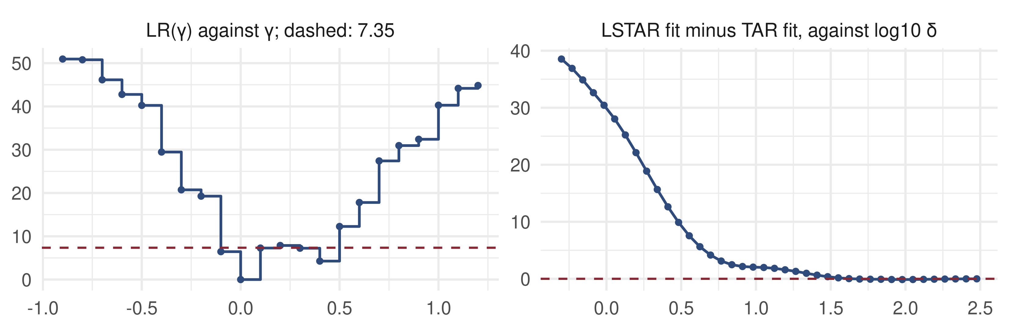
gamma_hat: 0   95% LR set: -0.1 0 0.1 0.3 0.4 
sup F: 55.5   bootstrap 95% point: 12.2   p-value: 0 
LSTAR best delta: 95.2   s2 LSTAR: 0.0367   s2 TAR: 0.03671 

Three answers: the LR set, the sup-F p-value, and the \(\delta\) the data choose.

💰 Case Study: What the Data Say

What the data say: the 95% set is disjoint, \(\{-0.1,0,0.1\}\cup\{0.3,0.4\}\). Linearity is rejected far beyond the bootstrap critical value. Right: \(T(\hat\sigma^2_{\text{LSTAR}}-\hat\sigma^2_{\text{TAR}})/\hat\sigma^2_{\text{TAR}}\) falls to zero only for large \(\delta\); with \(q\) recorded to one decimal, a steep dimmer and a switch fit alike.

📝 Quiz #1: The LR Set

\(LR(\gamma)\) takes the values 9.1, 6.2, 0, 3.4, 8.0, 5.1 on six consecutive grid points. Which points are in the 95% confidence set?

• The 2nd, 3rd, 4th and 6th
• The 2nd, 3rd and 4th only, since a confidence set must be an interval
• All six, since \(\hat\gamma\) is superconsistent
• The 3rd only

📝 Quiz #2: Critical Value

What is the 90% critical value \(c_{0.90}\) of \(\xi\), from \(\Pr\{\xi\le u\}=(1-e^{-u/2})^2\)?

• \(-2\ln(1-\sqrt{0.9})\approx5.94\)
• \(-2\ln(0.1)\approx4.61\)
• \(2.71\), the \(\chi^2(1)\) value
• \(\sqrt{0.9}\approx0.95\)

📝 Quiz #3: Limits of LSTAR

In an LSTAR model with logistic \(G(u,\gamma,\delta)\), what happens as \(\delta\to0\)?

• \(G\to\tfrac12\) and the model becomes a linear AR
• \(G\) becomes the indicator and the model becomes a TAR
• \(G\to0\) and only regime 1 remains
• The model becomes an ESTAR

📋 Key Formulas

LR statistic	\(LR(\gamma)=T\{\hat\sigma^2(\gamma)-\hat\sigma^2\}/\hat\sigma^2\)
Hansen’s limit	\(LR(\gamma_0)\xrightarrow{d}\xi=\max_r\{2B(r)-\lvert r\rvert\}\), \(\Pr\{\xi\le u\}=(1-e^{-u/2})^2\)
critical values	\(c_{1-\alpha}=-2\ln(1-\sqrt{1-\alpha})\): 5.94, 7.35, 10.59
confidence set	\(\{\gamma:LR(\gamma)\le c_{1-\alpha}\}\)
sup-F	\(\max_\gamma T\{\tilde\sigma^2-\hat\sigma^2(\gamma)\}/\hat\sigma^2(\gamma)\), fixed-regressor bootstrap
STAR	\(x_t=(\mu_1+\rho_1x_{t-1})(1-G)+(\mu_2+\rho_2x_{t-1})G+\varepsilon_t\)
LSTAR / ESTAR	\([1+e^{-\delta(u-\gamma)}]^{-1}\) / \(1-e^{-\delta(u-\gamma)^2}\)

📋 Summary

• Under shrinking threshold effects, \(LR(\gamma_0)\) has a pivotal limit with a closed-form CDF
• Inverting \(LR(\gamma)\) gives a confidence set that may be asymmetric or disjoint
• Under linearity \(\gamma\) is unidentified: use sup-F with bootstrap critical values, never \(\chi^2\)
• The fixed-regressor bootstrap keeps the regressors and redraws only the dependent variable
• STAR models blend the regimes with \(G\in[0,1]\); \(\delta\) runs from linear (\(0\)) to TAR (\(\infty\))

📚 Further Reading

• Hansen, B. E. (2000), “Sample splitting and threshold estimation”, Econometrica
• Hansen, B. E. (1996), “Inference when a nuisance parameter is not identified under the null hypothesis”, Econometrica
• Davies, R. B. (1977, 1987), Biometrika; Andrews, D. W. K. and Ploberger, W. (1994), Econometrica
• Teräsvirta, T. (1994), “Specification, estimation, and evaluation of smooth transition autoregressive models”, JASA
• Franses, P. H. and van Dijk, D. (2000), Non-linear Time Series Models in Empirical Finance, ch. 3

Next lecture: Markov Switching and State-Space Models. Regimes driven not by an observed threshold variable but by a hidden state.

⬅ Previous lecture: 11 · Nonlinear Models and Threshold Autoregression