Time Series Econometrics

Lecture 13: Markov Switching and State-Space Models

Samir Orujov, PhD

Open lecture notes, after Stanislav Anatolyev’s course (2016)

🎬 The Idea in 3 Minutes

⬅ Previous lecture: 12 · Threshold Inference and Smooth Transition

A short film with the intuition. Watch it before the slides, or after. Captions: CC button.

🎯 Learning Objectives

By the end of this lecture, you will be able to:

  • Test linearity against a smooth transition model with a Taylor-expansion auxiliary regression
  • Write down a two-state Markov switching autoregression and read its transition matrix
  • Run the Hamilton filter by hand: predict, observe, update
  • Estimate the model by maximum likelihood and interpret filtered regime probabilities
  • Describe a state-space model by its observation and transition equations

🔁 Warm-up from last time

Last lecture we tested a linear AR(1) against a threshold AR with the statistic \(\sup_{\gamma\in\Gamma}F(\gamma)\). Why can its critical values not be read from a \(\chi^2\) or \(F\) table?

  • Under \(H_0\) the threshold \(\gamma\) does not enter the model, so it is not identified
  • Because the errors are heteroskedastic
  • Because \(\hat\gamma\) converges at rate \(T\) rather than \(\sqrt T\)
  • Because the sample is trimmed at the ends of the grid

🗺️ Where We Are

Lecture 12 ended with the smooth transition autoregression (STAR): \[x_t=(\mu_1+\rho_1x_{t-1})\{1-G\}+(\mu_2+\rho_2x_{t-1})\,G+\varepsilon_t,\qquad G=G\big(\delta(x_{t-1}-\gamma)\big).\]

In both TAR and STAR the regime is decided by something we see: the lagged value \(x_{t-1}\) against a threshold \(\gamma\).

Today: first, how to test linearity in STAR without the sup-F machinery. Then the step to a regime we never see, which moves by its own probabilistic law.

❓ The Question

Is the economy in a recession right now?

The NBER dates US recessions months, sometimes more than a year, after they begin. Yet a forecaster, a central bank or a bond desk must act on the current quarter’s GDP figure.

Suppose growth behaves differently in expansions and recessions, and the regime itself is hidden. Can the data alone tell us, quarter by quarter, the probability that we are in a recession?

🧪 Testing Linearity in STAR

Linearity is \[H_0:\ \mu_1=\mu_2,\ \rho_1=\rho_2 .\]

Under \(H_0\) the transition function multiplies zero, so \(\gamma\) and \(\delta\) do not enter the likelihood. They are not identified, and Wald, LR and LM statistics lose their \(\chi^2\) limits: the problem of Lecture 12 again.

Equivalently \(H_0:\delta=0\), since \(G(0)=\tfrac12\) is constant. Under this form the unidentified parameters are \(\gamma\) and the differences \(\mu_2-\mu_1\), \(\rho_2-\rho_1\).

Remedy: replace \(G\) by a Taylor polynomial in \(\delta\) around \(\delta=0\). The unidentified parameters are absorbed into coefficients of an ordinary regression.

🧪 The Auxiliary Regression

For the logistic \(G(u)=[1+e^{-u}]^{-1}\), around \(u=0\): \(G(u)\approx\tfrac12+\tfrac14u-\tfrac1{48}u^3\), with \(u=\delta(x_{t-1}-\gamma)\).

Write the STAR model as \(x_t=\mu_1+\rho_1x_{t-1}+\big[(\mu_2-\mu_1)+(\rho_2-\rho_1)x_{t-1}\big]G+\varepsilon_t\). Substituting the cubic in \(x_{t-1}\) and multiplying by the linear bracket gives a quartic in \(x_{t-1}\): \[x_t=\mu+\rho x_{t-1}+\beta_1x_{t-1}^2+\beta_2x_{t-1}^3+\beta_3x_{t-1}^4+e_t .\]

Each \(\beta_k\) is proportional to \(\delta\) (or \(\delta^3\)), so linearity becomes \[\tilde H_0:\ \beta_1=\beta_2=\beta_3=0,\qquad W\xrightarrow[H_0]{d}\chi^2_{3}.\] This is the test of Luukkonen, Saikkonen and Teräsvirta (1988).

💻 The Taylor Test in R

Code
lin_test <- function(x) {                     # Wald test of beta1 = beta2 = beta3 = 0
  y <- x[-1]; z <- x[-length(x)]
  X <- cbind(1, z, z^2, z^3, z^4)
  b <- solve(crossprod(X), crossprod(X, y)); e <- y - X %*% b
  V <- sum(e^2) / (length(y) - 5) * solve(crossprod(X))
  W <- drop(t(b[3:5]) %*% solve(V[3:5, 3:5]) %*% b[3:5])
  c(W = W, p_value = pchisq(W, df = 3, lower.tail = FALSE))
}
n_obs <- 400; e <- rnorm(n_obs); x_lin <- x_star <- numeric(n_obs)
for (t in 2:n_obs) {
  x_lin[t] <- 0.5 + 0.6 * x_lin[t - 1] + e[t]
  G <- plogis(3 * (x_star[t - 1] - 1))         # LSTAR, gamma = 1, delta = 3
  x_star[t] <- (0.5 + 0.8 * x_star[t - 1]) * (1 - G) + (-1 + 0.2 * x_star[t - 1]) * G + e[t]
}
rbind(linear_AR = lin_test(x_lin), LSTAR = lin_test(x_star)) |> round(4)
                 W p_value
linear_AR   0.8026  0.8488
LSTAR     114.9548  0.0000

Same shocks, same length: the test is silent on the linear AR and rejects for the LSTAR.

🔀 Markov Switching Autoregression

Two-state MSW-AR(1)

\[x_t=\begin{cases}\mu_1+\rho_1x_{t-1} & \text{if } s_t=1\\ \mu_2+\rho_2x_{t-1} & \text{if } s_t=2\end{cases}\;+\;\varepsilon_t,\qquad \varepsilon_t\mid I_{t-1}\sim N(0,\sigma^2).\] The state \(s_t\in\{1,2\}\) is unobservable.

In TAR the switch was an observable event, \(x_{t-d}\) crossing \(\gamma\). Here we never see the switch. What we do know is the law of motion of \(s_t\).

⛓️ The Markov Chain for \(s_t\)

\(s_t\) is a first-order Markov chain with transition matrix \[P=\begin{pmatrix}p & 1-p\\ 1-q & q\end{pmatrix},\qquad P_{ij}=\Pr(s_{t+1}=j\mid s_t=i).\] \(p\) is the probability of staying in state 1; \(1-p\) is the probability of switching from 1 to 2.

  • Ergodic probabilities solve \(\pi_1=p\,\pi_1+(1-q)\pi_2\), \(\pi_1+\pi_2=1\): \[\pi_1=\frac{1-q}{2-p-q},\qquad \pi_2=\frac{1-p}{2-p-q}.\]
  • Duration of a spell in state 1: \(\Pr(D=k)=p^{k-1}(1-p)\), a geometric law, so \(E[D]=1/(1-p)\).

🎛️ Explore: Persistence and Durations

🧩 Extensions

The two-state AR(1) is the simplest member of a large family:

  • higher autoregressive order, \(x_t=\mu_{s_t}+\rho_{1,s_t}x_{t-1}+\dots+\rho_{k,s_t}x_{t-k}+\varepsilon_t\)
  • regime-wise heteroskedasticity, \(\varepsilon_t\mid I_{t-1},s_t\sim N(0,\sigma^2_{s_t})\)
  • more than two states, with an \(M\times M\) transition matrix
  • higher-order Markov chains for \(s_t\)

Every extension keeps the same estimation logic, which we now develop.

📐 Estimation: The Likelihood

If we knew \(f(x_t\mid I_{t-1})\) we would apply MLE. Conditional on the state it is simple: \[f(x_t\mid I_{t-1},s_t=j)=\frac1\sigma\,\phi\!\left(\frac{x_t-\mu_j-\rho_jx_{t-1}}{\sigma}\right),\qquad j\in\{1,2\}.\]

But \(s_t\) is unobservable, so we integrate it out. By total probability, \[f(x_t\mid I_{t-1})=\sum_{j=1}^2 f(x_t\mid I_{t-1},s_t=j)\,\Pr(s_t=j\mid I_{t-1}).\] The density is a mixture of two normals with time-varying weights. Everything hinges on the predicted probabilities \(\Pr(s_t=j\mid I_{t-1})\).

🔁 The Hamilton Filter

Update (Bayes, with \(I_t=\{x_t,I_{t-1}\}\)): \[\Pr(s_t=j\mid I_t)=\frac{f(x_t\mid s_t=j,I_{t-1})\,\Pr(s_t=j\mid I_{t-1})}{\sum_{i=1}^2 f(x_t\mid s_t=i,I_{t-1})\,\Pr(s_t=i\mid I_{t-1})}.\]

Predict (total probability): \[\Pr(s_{t+1}=j\mid I_t)=\sum_{i=1}^2\Pr(s_{t+1}=j\mid s_t=i)\,\Pr(s_t=i\mid I_t)=\sum_{i=1}^2P_{ij}\,\Pr(s_t=i\mid I_t).\] By the Markov property, \(I_t\) drops out of the transition probability, which is an element of \(P\).

The predicted probabilities feed the next update. Run the recursion from the beginning of the sample to the end, starting from the ergodic probabilities \(\pi_1,\pi_2\).

📐 Maximum Likelihood

\[\theta=(\mu_1,\rho_1,\mu_2,\rho_2,\sigma^2,p,q),\qquad \hat\theta=\arg\max_\theta\ \frac1T\sum_{t=1}^T\log f(x_t\mid I_{t-1}).\] The denominator of each update step is \(f(x_t\mid I_{t-1})\), so one pass of the filter evaluates the likelihood.

  • With \(p,q<1\) and two distinct regimes, \(\hat\theta\) has standard asymptotics: consistent and asymptotically normal, with the usual inverse-Hessian variance.
  • If \(p=1\) (or \(q=1\)) the state is absorbing: once the system falls in that regime, it stays there forever.
  • Testing one regime against two is non-standard: under \(H_0\), \(p\) and \(q\) are not identified, as \(\gamma\) was in TAR.

✍️ Worked Example: One Filter Step

Take \(\mu_1=1.1\), \(\rho_1=0.15\), \(\mu_2=-0.3\), \(\rho_2=0.05\), \(\sigma=0.9\), \(p=0.90\), \(q=0.70\). Last quarter \(x_{t-1}=0.2\); the filter predicts \(\Pr(s_t=1\mid I_{t-1})=0.80\). Growth comes in at \(x_t=-0.6\).

1. Conditional means. \(1.1+0.15(0.2)=1.13\) and \(-0.3+0.05(0.2)=-0.29\).

2. Densities. \(f_1=\phi\big(\tfrac{-0.6-1.13}{0.9}\big)/0.9=\phi(-1.922)/0.9=0.0699\); \(f_2=\phi(-0.344)/0.9=0.4177\).

3. Update. \(\Pr(s_t=1\mid I_t)=\dfrac{0.80(0.0699)}{0.80(0.0699)+0.20(0.4177)}=\dfrac{0.0559}{0.1394}=0.401\).

4. Predict. \(\Pr(s_{t+1}=1\mid I_t)=0.90(0.401)+0.30(0.599)=0.541\).

💻 The Same Step in R

Code
mu <- c(1.1, -0.3); rho <- c(0.15, 0.05); sigma <- 0.9
P  <- matrix(c(0.90, 0.10,
               0.30, 0.70), 2, byrow = TRUE)   # rows: from state i
prior <- c(0.80, 0.20); x_prev <- 0.2; x_now <- -0.6
f    <- dnorm(x_now, mean = mu + rho * x_prev, sd = sigma)
post <- f * prior / sum(f * prior)                 # update
pred <- as.vector(t(P) %*% post)                   # predict
list(densities = round(f, 4), likelihood_contribution = round(sum(f * prior), 4),
     filtered = round(post, 3), predicted_next = round(pred, 3))
$densities
[1] 0.0699 0.4177

$likelihood_contribution
[1] 0.1394

$filtered
[1] 0.401 0.599

$predicted_next
[1] 0.541 0.459

One bad quarter halves the probability of expansion, from 0.80 to 0.40. The chance of leaving the recession state, \(1-q=0.3\), lifts next quarter’s forecast to 0.54.

💻 The Filter as a Loop

Code
hamilton <- function(theta, x, filtered = FALSE) {
  mu <- theta[1:2]; rho <- theta[3:4]; sigma <- exp(theta[5])      # sigma > 0
  p <- plogis(theta[6]); q <- plogis(theta[7])                     # p, q in (0, 1)
  P <- matrix(c(p, 1 - p, 1 - q, q), 2, byrow = TRUE)
  pred <- c(1 - q, 1 - p) / (2 - p - q)                            # ergodic start
  filt <- matrix(NA, length(x), 2); loglik <- 0
  for (t in 2:length(x)) {
    num <- dnorm(x[t], mu + rho * x[t - 1], sigma) * pred
    loglik <- loglik + log(sum(num))                               # log f(x_t | I_{t-1})
    filt[t, ] <- num / sum(num)                                    # update
    pred <- as.vector(t(P) %*% filt[t, ])                          # predict
  }
  if (filtered) filt else -loglik                                  # optim minimises
}

The parameters are mapped to an unrestricted scale (\(\log\sigma\), logits of \(p,q\)) so that optim can search freely.

📈 Filtered Probabilities, Simulated

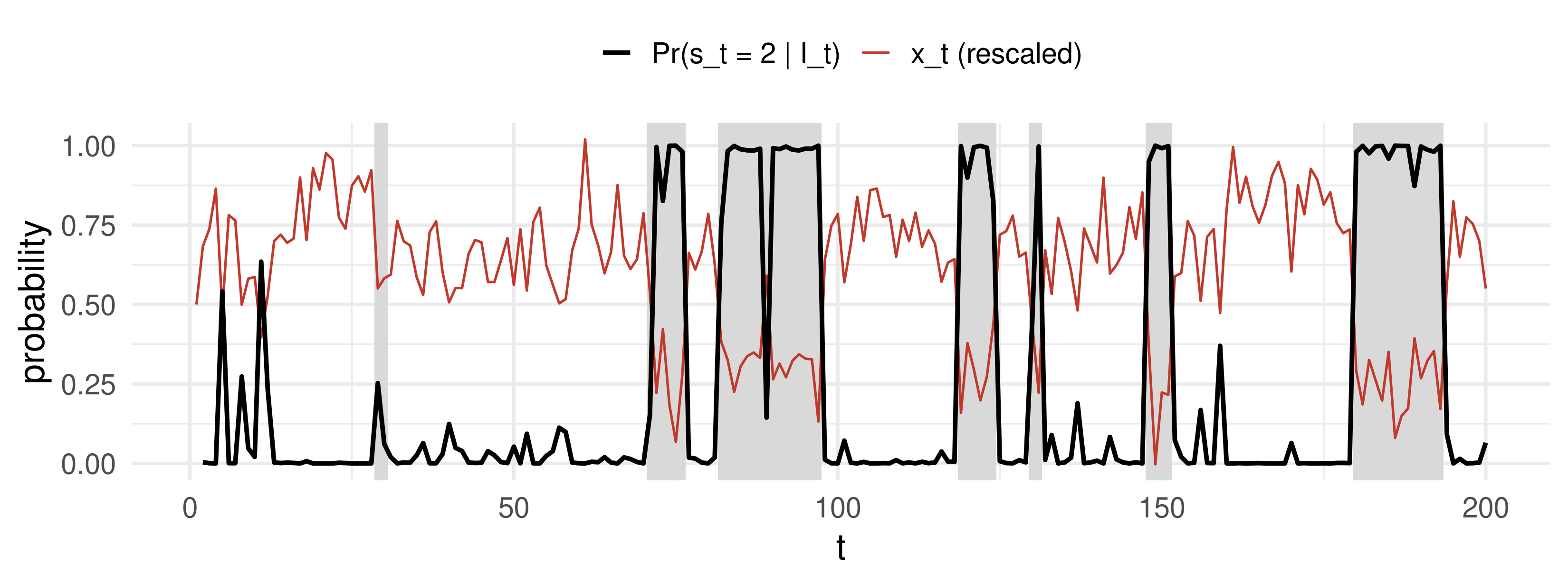
Grey bands mark the true state 2. The filtered probability (black) jumps between near 0 and near 1 and identifies the regime periods, with a short lag at each switch.

🧠 Think-Pair-Share

A quarterly MSW model has expansion state 1 and recession state 2, with \(p=0.95\) and \(q=0.80\).

  1. What fraction of quarters does the economy spend in recession in the long run?
  2. How long does a typical recession last? A typical expansion?
  3. This quarter \(\Pr(s_t=2\mid I_t)=0.6\). What is \(\Pr(s_{t+1}=2\mid I_t)\)?
  4. What changes if \(q=1\)?

✅ Think-Pair-Share: Solution

  1. \(\pi_2=\dfrac{1-p}{2-p-q}=\dfrac{0.05}{0.25}=0.20\): one quarter in five.
  2. Recessions last \(1/(1-q)=5\) quarters on average; expansions \(1/(1-p)=20\) quarters.
  3. Predict step: \(\Pr(s_{t+1}=2\mid I_t)=(1-p)(0.4)+q(0.6)=0.02+0.48=0.50\).
  1. With \(q=1\) state 2 is absorbing: \(\pi_2=0.05/0.05=1\). The first recession never ends, and the model forecasts a recession at every long horizon.

🏗️ State-Space Models

Markov switching is one model with a latent variable. The general class, the state-space model, has two parts:

  1. Observation equation: links the observable variables to the unobservable ones.
  2. Transition equation: the dynamics of the latent variable. We do not see it, but we know how it moves.

In the MSW model the observation equation is \(x_t=\mu_{s_t}+\rho_{s_t}x_{t-1}+\varepsilon_t\), and the transition equation is the Markov chain \(P\). For a continuous latent state with linear Gaussian dynamics, the analogue of the Hamilton filter is the Kalman filter.

Not in the 2016 notes: the Kalman filter remark is added from Hamilton (1994), ch. 13 and 22.

🏗️ Example: Giordani and Villani (2008)

Observation equation: \(\;y_t=\mu_t+x_t+\varepsilon_t\), with \(\mu_t\) a local mean.

Transition of the local mean, \(u_{\mu,t}\sim N(0,1)\): \[\mu_t=\begin{cases}\bar\mu+\sigma_{\mu,1}u_{\mu,t} & \text{w.p. } \pi_1 \quad\text{(a break to a new level)}\\ \mu_{t-1}+\sigma_{\mu,2}u_{\mu,t} & \text{w.p. } \pi_2 \quad\text{(a small shift)}\\ \mu_{t-1} & \text{w.p. } 1-\pi_1-\pi_2 \quad\text{(no change)}\end{cases}\]

Transitory part: \(x_t=\rho_1x_{t-1}+\dots+\rho_px_{t-p}+u_{x,t}\), with \(u_{x,t}\) a mixture of \(K_x\) normals (weights \(\pi_x\), means \(\alpha_x\), variances \(\sigma^2_{x,t}\xi_x^2\)).

🏗️ Volatility That Moves Rarely

The scale of the transitory shocks is itself a latent state: \[\log\sigma_{x,t}=\begin{cases}\log\sigma_{x,t-1}+\sigma_x e_{x,t} & \text{w.p. } \pi_x^\sigma\\ \log\sigma_{x,t-1} & \text{w.p. } 1-\pi_x^\sigma\end{cases},\qquad e_{x,t}\sim\text{iid }N(0,1).\]

The level and the volatility each switch between “move” and “stay” with their own probabilities, and the transitory shock is a mixture of normals. One model then accommodates level breaks, outliers and volatility shifts, and the filter tells us at each date which of them most likely occurred.

💰 Case Study: Recessions from GDP

📈 The question

Fit the two-state MSW-AR(1) to US real GDP growth by maximum likelihood.

  1. Does one state have negative mean growth?
  2. How persistent are the two states?
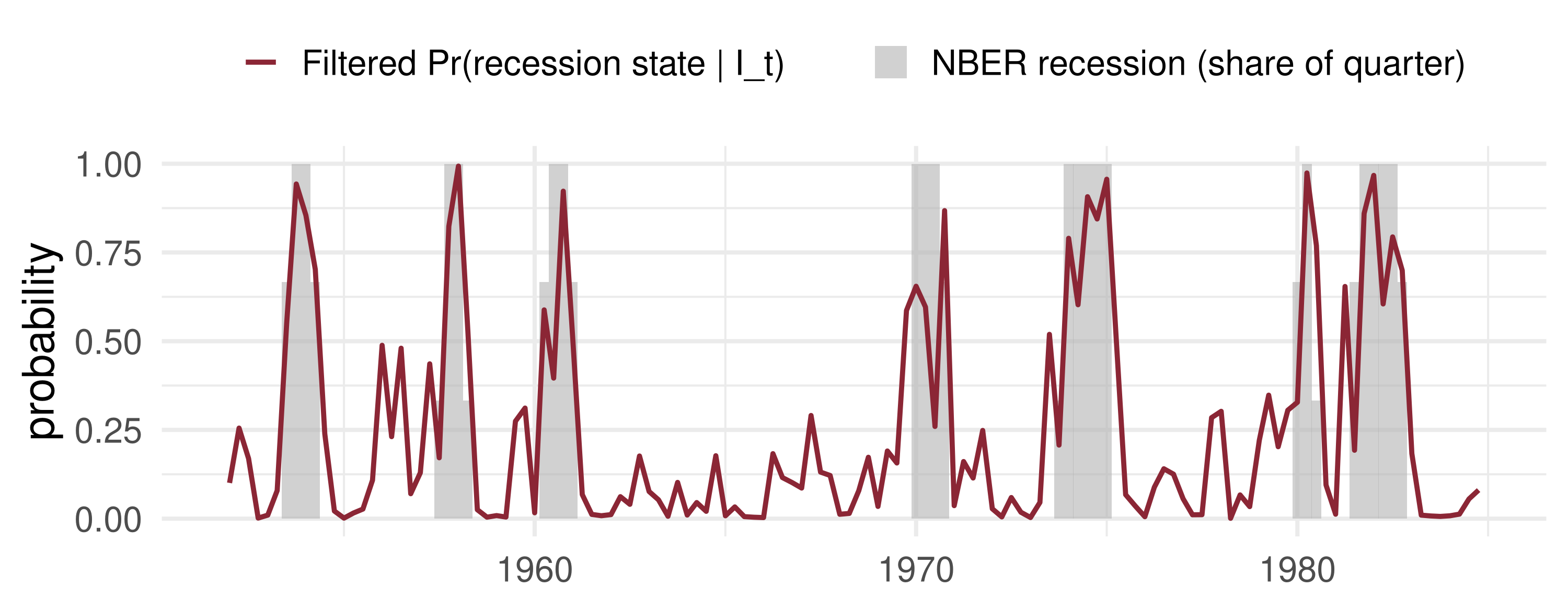
  3. Do the filtered recession probabilities line up with NBER recessions?

📊 The data

Series: real GDP (FRED GDPC1); NBER recession indicator (FRED USREC)

Period: 1952Q1–1984Q4, the sample of Hamilton (1989)

\(x_t=100\,\Delta\log \text{GDP}_t\), quarterly per cent

gdp <- read.csv("https://fred.stlouisfed.org/graph/fredgraph.csv?id=GDPC1")
rec <- read.csv("https://fred.stlouisfed.org/graph/fredgraph.csv?id=USREC")

💰 Case Study: The MLE in R

📦 Load GDP, maximise the Hamilton-filter likelihood
g <- read.csv("data/GDPC1.csv"); g$date <- as.Date(g$observation_date)
x_all <- 100 * diff(log(g$GDPC1)); d_all <- g$date[-1]
use <- d_all >= as.Date("1951-10-01") & d_all <= as.Date("1984-10-01")  # first obs is a lag
x <- x_all[use]; d <- d_all[use]
start <- c(1, -0.5, 0.3, 0.3, log(0.8), qlogis(0.9), qlogis(0.7))
fit <- optim(start, hamilton, x = x, method = "BFGS", hessian = TRUE)
th  <- fit$par
se  <- sqrt(diag(solve(fit$hessian)))
est <- c(mu1 = th[1], mu2 = th[2], rho1 = th[3], rho2 = th[4], sigma = exp(th[5]),
         p = plogis(th[6]), q = plogis(th[7]))
use19 <- d_all >= as.Date("1951-10-01")                         # same model, to 2019Q4
fit19 <- optim(start, hamilton, x = x_all[use19], method = "BFGS")
list(estimates_1952_1984 = round(rbind(estimate = est, se = c(se[1:4], NA, NA, NA)), 3),
     mean_duration_qtrs  = round(c(expansion = 1 / (1 - est[["p"]]),
                                   recession = 1 / (1 - est[["q"]])), 2),
     p_q_if_sample_ends_2019 = round(c(p = plogis(fit19$par[6]), q = plogis(fit19$par[7])), 3))
$estimates_1952_1984
           mu1    mu2  rho1  rho2 sigma     p     q
estimate 1.072 -0.268 0.159 0.044  0.88 0.896 0.697
se       0.229  0.316 0.111 0.247    NA    NA    NA

$mean_duration_qtrs
expansion recession 
     9.60      3.31 

$p_q_if_sample_ends_2019
    p     q 
0.951 0.195 

Look at \(\hat\mu_2<0\) (the recession state), at the mean durations, and at how \(\hat q\) changes when the sample runs to 2019.

💰 Case Study: Filter vs NBER

What the data say: using GDP alone, the filter picks out every NBER recession from 1953 to 1982, usually within a quarter. It fails on the post-1984 sample: re-estimated to 2019, the common \(\sigma\) must also fit the calmer Great Moderation, and the second state shrinks to short outlier quarters (the last line of the output); regime-specific variances are then needed.

📝 Quiz #1: The Predict Step

With \(p=0.9\), \(q=0.6\) and \(\Pr(s_t=1\mid I_t)=0.5\), what is \(\Pr(s_{t+1}=1\mid I_t)\)?

  • \(0.65\)
  • \(0.75\)
  • \(0.50\)
  • \(0.54\)

📝 Quiz #2: Ergodic Probabilities

A two-state chain has \(p=0.98\) and \(q=0.90\). What is the long-run share of time in state 2?

  • \(1/6\approx0.17\)
  • \(0.10\)
  • \(0.50\)
  • \(0.02\)

📝 Quiz #3: TAR vs Markov Switching

What is the essential difference between a TAR model and a Markov switching model?

  • In TAR the regime is determined by an observable variable crossing a threshold; in MSW the regime is a latent Markov chain
  • TAR allows two regimes, MSW allows only one
  • MSW requires regime-specific variances, TAR does not
  • TAR is estimated by MLE, MSW by least squares

📋 Key Formulas

STAR linearity test \(x_t=\mu+\rho x_{t-1}+\sum_{k=1}^3\beta_kx_{t-1}^{k+1}+e_t\), \(W\to\chi^2_3\)
Transition matrix \(P=\begin{pmatrix}p&1-p\\1-q&q\end{pmatrix}\)
Ergodic, duration \(\pi_1=\frac{1-q}{2-p-q}\), \(E[D_1]=\frac1{1-p}\)
Likelihood \(f(x_t\mid I_{t-1})=\sum_jf(x_t\mid s_t=j,I_{t-1})\Pr(s_t=j\mid I_{t-1})\)
Update \(\Pr(s_t=j\mid I_t)\propto f(x_t\mid s_t=j,I_{t-1})\Pr(s_t=j\mid I_{t-1})\)
Predict \(\Pr(s_{t+1}=j\mid I_t)=\sum_iP_{ij}\Pr(s_t=i\mid I_t)\)

📋 Summary

  • Linearity against STAR: Taylor-expand \(G\) around \(\delta=0\); a Wald test on \(x_{t-1}^2,x_{t-1}^3,x_{t-1}^4\) is \(\chi^2_3\)
  • In MSW the regime is a hidden Markov chain; \(p\) and \(q\) fix the persistence and the long-run shares
  • The likelihood is a mixture; the Hamilton filter supplies its weights by predict and update steps
  • \(\hat\theta\) has standard asymptotics when \(p,q<1\); the number of regimes is a non-standard test
  • State-space models: an observation equation plus a transition equation for the latent part

📚 Further Reading

  • Hamilton, J. D. (1989). A new approach to the economic analysis of nonstationary time series and the business cycle. Econometrica 57, 357–384.
  • Hamilton, J. D. (1994). Time Series Analysis, ch. 13 (Kalman filter) and ch. 22 (regime switching).
  • Luukkonen, R., Saikkonen, P. and Teräsvirta, T. (1988). Testing linearity against smooth transition autoregressive models. Biometrika 75, 491–499.
  • Franses, P. H. and van Dijk, D. (2000). Non-Linear Time Series Models in Empirical Finance, ch. 3.
  • Kim, C.-J. and Nelson, C. R. (1999). State-Space Models with Regime Switching.
  • Giordani, P. and Villani, M. (2008), the local-mean model with mixture shocks.

Next lecture: Vector Autoregressions, Impulse Responses and Cointegration.