Time Series Econometrics

🎬 The Idea in 3 Minutes

⬅ Previous lecture: 13 · Markov Switching and State-Space Models

A short film with the intuition. Watch it before the slides, or after. Captions: CC button.

🎯 Learning Objectives

By the end of this lecture, you will be able to:

Set up a VAR(\(p\)), check its stationarity, estimate it by OLS and choose its order
Compute orthogonalised impulse responses and a forecast error variance decomposition
Test Granger causality with an \(F\) test, and say what it does and does not mean
Recognise a spurious regression between two \(I(1)\) series
Distinguish it from a cointegrating regression, with economic examples

🔁 Warm-up from last time

In the Hamilton filter for a Markov switching AR, what is the denominator of the update step, \(\sum_i f(x_t\mid s_t=i,I_{t-1})\Pr(s_t=i\mid I_{t-1})\)?

The conditional density \(f(x_t\mid I_{t-1})\), the observation’s likelihood contribution
The ergodic probability of state 1
The transition probability \(p\)
The filtered probability \(\Pr(s_t=1\mid I_t)\)

🗺️ Where We Are

Lecture 13 ended with state-space models: one observed series, latent states behind it.

In Lecture 7 the Wold decomposition gave a univariate impulse response: the MA(\(\infty\)) weights of \(x_t\).

Today we model several series jointly. The questions become:

how does a shock to one variable move the others, and for how long?
which shocks explain most of each variable’s forecast errors?
what happens when the series are not stationary but \(I(1)\)?

❓ The Question

What does a monetary tightening do?

The central bank raises the policy rate by surprise. Inflation, unemployment and the rate itself all move, and each feeds back into the others.

A single equation cannot answer “what happens next quarter, and the quarter after?” because every variable is both cause and effect. We need a system in which each variable depends on the past of all of them.

📐 The VAR(\(p\)) Model

For an \(m\times1\) vector \(x_t\), \[x_t=a_0+A_1x_{t-1}+\dots+A_px_{t-p}+\varepsilon_t,\qquad E(\varepsilon_t\mid I_{t-1})=0,\quad \operatorname{var}(\varepsilon_t\mid I_{t-1})=\Sigma .\] Each \(A_j\) is \(m\times m\). Row \(k\) of the system is a regression of \(x_{k,t}\) on \(p\) lags of every variable.

The errors \(\varepsilon_t\) are the one-step forecast errors (innovations). They are serially uncorrelated but correlated with each other: \(\Sigma\) is not diagonal.

Bivariate example: \(x_t=(\Delta m_t,\Delta p_t)'\), money growth and inflation.

Not in the 2016 notes: added from Hamilton (1994), ch. 11, and Lütkepohl (2005), ch. 2.

📐 Stationarity of a VAR

Stack \(\xi_t=(x_t',x_{t-1}',\dots,x_{t-p+1}')'\). Then \(\xi_t=c+F\xi_{t-1}+(\varepsilon_t',0,\dots,0)'\) with the companion matrix \[F=\begin{pmatrix}A_1&A_2&\cdots&A_{p-1}&A_p\\ I_m&0&\cdots&0&0\\ \vdots&&\ddots&&\vdots\\ 0&0&\cdots&I_m&0\end{pmatrix}.\]

The VAR is (covariance) stationary if every eigenvalue of \(F\) lies inside the unit circle; equivalently, all roots of \[\det\big(I_m-A_1z-\dots-A_pz^p\big)=0\] lie outside it. This is the vector version of the AR(\(p\)) root condition.

Not in the 2016 notes: added from Hamilton (1994), ch. 10.

📐 Estimation by OLS

Every equation has the same regressors \(z_t=(1,x_{t-1}',\dots,x_{t-p}')'\). Write \(x_t=Bz_t+\varepsilon_t\); then \[\hat B'=\Big(\sum_t z_tz_t'\Big)^{-1}\sum_t z_tx_t',\qquad \hat\Sigma=\frac1T\sum_t\hat\varepsilon_t\hat\varepsilon_t' .\]

With identical regressors, OLS on each equation separately equals GLS on the system and the Gaussian MLE, despite the correlated errors (Zellner’s SUR result).
Under stationarity, \(\hat B\) is consistent and asymptotically normal; the usual OLS \(t\), \(F\) and Wald tests apply equation by equation.

Not in the 2016 notes: added from Hamilton (1994), ch. 11.

📐 Choosing the Lag Order

Fit VAR(\(p\)) for \(p=1,\dots,p_{\max}\) on a common sample and minimise \[\text{AIC}(p)=\log\det\hat\Sigma_p+\frac{2pm^2}{T},\qquad \text{BIC}(p)=\log\det\hat\Sigma_p+\frac{pm^2\log T}{T},\] \[\text{HQ}(p)=\log\det\hat\Sigma_p+\frac{2pm^2\log\log T}{T}.\]

The trade-off of Lecture 4 in matrix form: \(\log\det\hat\Sigma_p\) falls with \(p\), the penalty grows with the \(pm^2\) coefficients. BIC and HQ choose the true order with probability tending to one; AIC tends to overfit but often forecasts well.

Not in the 2016 notes: added from Lütkepohl (2005), ch. 4.

📐 Orthogonal Shocks

A stable VAR has the MA(\(\infty\)) form \(x_t=\mu+\sum_{s\ge0}\Phi_s\varepsilon_{t-s}\), with \(\Phi_0=I_m\) and \(\Phi_s=\sum_{j=1}^{\min(s,p)}A_j\Phi_{s-j}\).

Because \(\Sigma\) is not diagonal, “a shock to \(\varepsilon_1\) with \(\varepsilon_2\) fixed” never happens. Factor \[\Sigma=LDL',\qquad L \text{ lower triangular with unit diagonal},\quad D=\operatorname{diag}(\sigma_1^2,\dots,\sigma_m^2),\] and define \(v_t=L^{-1}\varepsilon_t\): orthogonal shocks with \(\operatorname{var}(v_t)=D\). Then \[x_t=\mu+\sum_{s\ge0}\Psi_sv_{t-s},\qquad \Psi_s=\Phi_sL .\]

This is the Cholesky (recursive) identification: the variable ordered first does not respond on impact to the shocks ordered after it.

Not in the 2016 notes: the factorisation is added from Hamilton (1994), ch. 11.

📈 Impulse Response Functions

\[\underset{m\times m}{\mathrm{IRF}(h)}=\frac{\partial x_{t+h}}{\partial v_t'}=\Psi_h .\] Element \((j,i)\) is the response of variable \(j\), \(h\) periods later, to a unit orthogonal shock \(v_i\) at time \(t\).

For \(x_t=(\Delta m_t,\Delta p_t)'\) with \(\Delta m\) ordered first:

own responses start at 1; money growth dies out with a damped oscillation, inflation monotonically
\(\Delta m\) does not react to the price shock \(v_p\) on impact; it rises to a hump later
in a stable VAR every response decays to zero

🎛️ Explore: Feedback and IRF Shape

Code

html`<div style="font-size:28px"><b style='color:#8b2635'>x₁ own</b> and <b style='color:#2f4b7c'>x₂ cross</b> response · A = [0.5, a₁₂; 0.6, 0.5], Σ = I · largest |eigenvalue| <b>${modulus.toFixed(3)}</b> · roots are <b>${disc < 0 ? "complex: oscillation" : "real: monotone decay"}</b>${modulus >= 1 ? " · <b style='color:#8b2635'>not stable</b>" : ""}</div>`

✍️ Worked Example: IRF by Hand

VAR(1) for \((\Delta m_t,\Delta p_t)'\): \(A=\begin{pmatrix}0.5&0.2\\0.3&0.4\end{pmatrix}\), \(\Sigma=\begin{pmatrix}1&0.5\\0.5&2\end{pmatrix}\).

Factor. \(L=\begin{pmatrix}1&0\\0.5&1\end{pmatrix}\), \(D=\operatorname{diag}(1,\ 2-0.5^2)=\operatorname{diag}(1,1.75)\). Check: \(LDL'=\Sigma\).

Responses. \(\Psi_0=L\); \(\ \Psi_1=AL=\begin{pmatrix}0.5+0.1&0.2\\0.3+0.2&0.4\end{pmatrix}=\begin{pmatrix}0.6&0.2\\0.5&0.4\end{pmatrix}\).

A money shock raises inflation by 0.5 on impact and 0.5 a quarter later; a price shock leaves \(\Delta m\) unchanged on impact and raises it by 0.2 after one quarter.

Granger. The (1,2) element of \(A\) is \(0.2\neq0\), so \(\Delta p\) Granger-causes \(\Delta m\); and \(0.3\neq0\), so \(\Delta m\) Granger-causes \(\Delta p\).

📊 Variance Decomposition (FEVD)

The \(h\)-step forecast error is \(x_{t+h}-E_tx_{t+h}=\sum_{s=0}^{h-1}\Psi_sv_{t+h-s}\). With orthogonal shocks, \[\operatorname{var}_t(x_{j,t+h})=\sum_{i=1}^m f_{ij}(h)\,\sigma_i^2,\qquad f_{ij}(h)=\sum_{s=0}^{h-1}(\Psi_s)_{ji}^2 .\] These are the diagonal elements of \(\operatorname{var}_t x_{t+h}\). The share of shock \(i\) in variable \(j\): \[\omega_{ij}(h)=\frac{f_{ij}(h)\,\sigma_i^2}{\sum_{k=1}^m f_{kj}(h)\,\sigma_k^2}\times100\%,\qquad \sum_i\omega_{ij}(h)=100\% .\]

Example above, \(h=2\), \(j=\Delta m\): \(f_{11}=1^2+0.6^2=1.36\), \(f_{21}=0^2+0.2^2=0.04\). Share of the money shock \(=\dfrac{1.36}{1.36+0.04\times1.75}=\dfrac{1.36}{1.43}=95.1\%\).

💻 The Example in R

Code

A <- matrix(c(0.5, 0.2,
              0.3, 0.4), 2, byrow = TRUE)
Sigma <- matrix(c(1, 0.5, 0.5, 2), 2)
C <- t(chol(Sigma))                       # Sigma = C C', C lower triangular
L <- C %*% diag(1 / diag(C))              # unit diagonal
D <- diag(diag(C)^2)                      # Sigma = L D L'
Psi <- list(L, A %*% L)                   # Psi_0, Psi_1
f   <- Reduce(`+`, lapply(Psi, function(P) P^2))   # f_ij(2), rows = variable j
share <- 100 * (f %*% D) / rowSums(f %*% D)
dimnames(share) <- list(c("dm", "dp"), c("v_m", "v_p"))
Psi_01 <- cbind(Psi[[1]], Psi[[2]]); colnames(Psi_01) <- c("Psi0_m", "Psi0_p", "Psi1_m", "Psi1_p")
list(D = diag(D), Psi_0_and_Psi_1 = Psi_01, FEVD_h2_percent = round(share, 1))

$D
[1] 1.00 1.75

$Psi_0_and_Psi_1
     Psi0_m Psi0_p Psi1_m Psi1_p
[1,]    1.0      0    0.6    0.2
[2,]    0.5      1    0.5    0.4

$FEVD_h2_percent
    v_m  v_p
dm 95.1  4.9
dp 19.8 80.2

🔎 Granger Causality

Definition

\(\Delta m\) does not Granger-cause \(\Delta p\) (\(\Delta m\overset{GC}{\not\to}\Delta p\)) if \[E(\Delta p_{t+1}\mid \Delta p_t,\Delta p_{t-1},\dots,\Delta m_t,\Delta m_{t-1},\dots)=E(\Delta p_{t+1}\mid \Delta p_t,\Delta p_{t-1},\dots).\]

In a VAR: all \(p\) coefficients on lagged \(\Delta m\) in the \(\Delta p\) equation are zero. Test this with an \(F\) (or Wald) statistic, \(F\sim F(p,\,T-mp-1)\) approximately.

It is a statistical notion, not an economic one. Stock prices Granger-cause dividends, because prices are forward-looking; economically, it is expected dividends that determine prices.

🧠 Think-Pair-Share

A VAR(1) has \(A=\begin{pmatrix}0.7&0\\0.5&0.2\end{pmatrix}\) and \(\Sigma=\begin{pmatrix}1&0.3\\0.3&1\end{pmatrix}\), with \(x_1\) ordered first.

Is the VAR stationary?
Which variable Granger-causes which?
Compute \(\Psi_0\) and \(\Psi_1\).
What share of the \(h\)-step forecast error variance of \(x_1\) comes from \(v_2\), for any \(h\)?

✅ Think-Pair-Share: Solution

\(A\) is triangular: eigenvalues \(0.7\) and \(0.2\), both inside the unit circle. Stationary.
\(a_{21}=0.5\neq0\): \(x_1\) Granger-causes \(x_2\). \(a_{12}=0\): \(x_2\) does not Granger-cause \(x_1\).
\(L=\begin{pmatrix}1&0\\0.3&1\end{pmatrix}\), \(D=\operatorname{diag}(1,0.91)\). \(\Psi_0=L\), \(\Psi_1=AL=\begin{pmatrix}0.7&0\\0.56&0.2\end{pmatrix}\).

Zero. \(x_1\) does not respond to \(v_2\) on impact (it is ordered first) and \(A\) never feeds \(x_2\) back into \(x_1\), so \((\Psi_s)_{12}=0\) for all \(s\). Its forecast errors are entirely its own shock.

⚠️ Spurious Regression

Let \(x_t,y_t\sim I(1)\) and run \(y_t=\beta x_t+\varepsilon_t\). There are two possibilities.

\(\varepsilon_t\sim I(1)\) for whatever \(\beta\): a spurious regression. OLS reports a large \(R^2\) and a “significant” \(t\), though there is no relation at all. Granger and Newbold’s example: rabbits in Australia against US GNP.
\(\varepsilon_t\sim I(0)\) for a certain \(\beta\): a cointegrating regression.

In case 1 the \(t\)-statistic does not converge to \(N(0,1)\); it diverges at rate \(\sqrt T\), and \(R^2\) converges to a random variable instead of to zero (Phillips, 1986). More data makes the illusion stronger.

💻 Two Independent Random Walks

Code

spurious <- function(n, reps = 1000) {
  out <- replicate(reps, {
    x <- cumsum(rnorm(n)); y <- cumsum(rnorm(n))        # independent I(1)
    s_lev <- summary(lm(y ~ x)); s_dif <- summary(lm(diff(y) ~ diff(x)))
    c(t_lev = s_lev$coefficients[2, 3], R2_lev = s_lev$r.squared,
      t_dif = s_dif$coefficients[2, 3])
  })
  c(T = n, reject_levels = mean(abs(out["t_lev", ]) > 1.96),
    median_R2 = median(out["R2_lev", ]), median_abs_t = median(abs(out["t_lev", ])),
    reject_differences = mean(abs(out["t_dif", ]) > 1.96))
}
sims <- t(sapply(c(50, 100, 200, 400, 800), spurious))
round(sims, 3)

       T reject_levels median_R2 median_abs_t reject_differences
[1,]  50         0.668     0.166        3.092              0.053
[2,] 100         0.763     0.192        4.826              0.056
[3,] 200         0.807     0.156        6.042              0.043
[4,] 400         0.894     0.168        8.966              0.054
[5,] 800         0.904     0.156       12.147              0.043

A nominal 5% test rejects two times in three at \(T=50\) and nine times in ten at \(T=800\); the median \(|t|\) grows like \(\sqrt T\). In first differences it rejects about 5% of the time, as it should.

📈 The \(t\)-Statistic Explodes

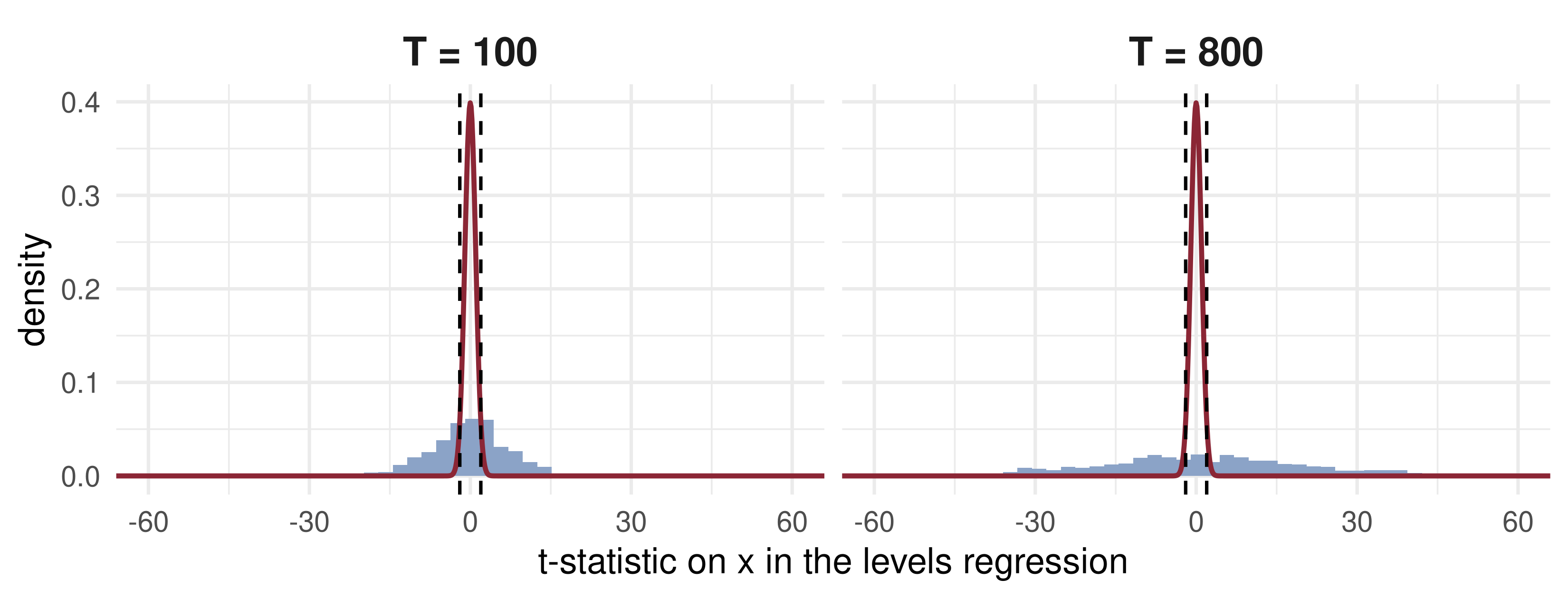
The red curve is the \(N(0,1)\) the textbook test assumes, squeezed inside the dashed lines. The actual spread is many times wider, and grows by about \(\sqrt8\approx2.8\) from \(T=100\) to \(T=800\).

🐕 The Drunk and Her Dog

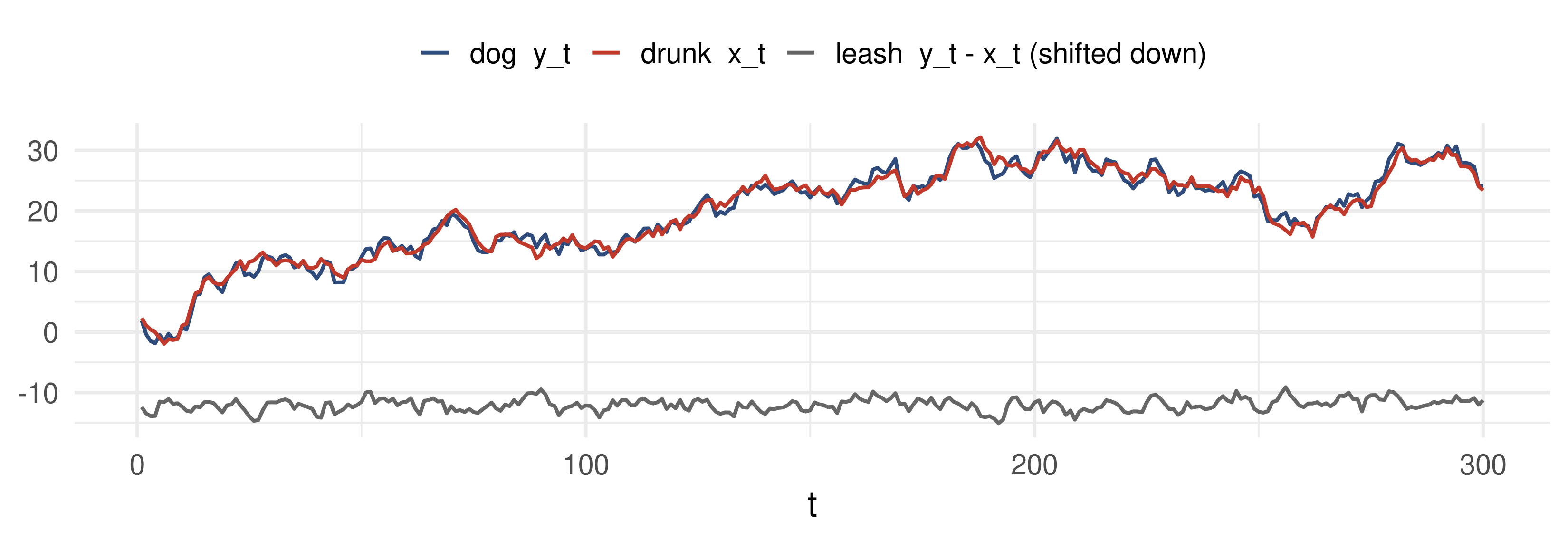
Each wanders like a random walk, but the leash keeps the distance \(y_t-x_t\) stationary: \(x_t,y_t\sim I(1)\) while \(y_t-\beta x_t\sim I(0)\) with \(\beta=1\). That is cointegration.

🌍 Cointegration in Economics

Known \(\beta\), implied by theory:

a constant consumption–income ratio: \(\log c_t-\log y_t\sim I(0)\), so the regression of \(\log c\) on \(\log y\) should be cointegrating
purchasing power parity: the real exchange rate \(e_t+p_t^*-p_t\sim I(0)\)
long and short interest rates: \(R_t-r_t\sim I(0)\)
spot and futures exchange rates

Unknown \(\beta\), to be estimated. Money demand: \[m_t-p_t=\alpha_1+\alpha_2y_t+\alpha_3r_t+I(0).\]

💰 Case Study: A Monetary Policy VAR

📈 The question

A VAR in inflation, unemployment and the federal funds rate, in the spirit of Stock and Watson (2001).

Which lag order do the criteria choose?
Does the policy rate Granger-cause inflation, and inflation the rate?
How do the three variables respond to a policy-rate shock?

📊 The data

Series: CPI (CPIAUCSL), unemployment rate (UNRATE), effective fed funds rate (FEDFUNDS), FRED

Period: 1960Q1–2007Q4, quarterly averages; ends before the zero lower bound

\(\pi_t=400\,\Delta\log\text{CPI}_t\); ordering \((\pi_t,u_t,R_t)\)

base <- "https://fred.stlouisfed.org/graph/fredgraph.csv?id="
raw  <- lapply(c("CPIAUCSL", "UNRATE", "FEDFUNDS"),
               function(i) read.csv(paste0(base, i)))

💰 Case Study: Estimation in R

📦 Data, lag order, OLS, Granger tests

qavg <- function(id) { z <- read.csv(paste0("data/", id, ".csv")); d <- as.Date(z$observation_date)
  tapply(z[[id]], paste(format(d, "%Y"), (as.numeric(format(d, "%m")) - 1) %/% 3 + 1), mean) }
cpi <- qavg("CPIAUCSL"); un <- qavg("UNRATE"); ff <- qavg("FEDFUNDS")
Y <- cbind(infl = 400 * diff(log(cpi)), u = un[-1], R = ff[-1])     # 1960Q1-2007Q4
m <- ncol(Y)
var_ols <- function(Y, p) {                       # OLS equation by equation
  n <- nrow(Y); Z <- cbind(1, do.call(cbind, lapply(1:p, function(j) Y[(p + 1 - j):(n - j), ])))
  X <- Y[(p + 1):n, ]; B <- solve(crossprod(Z), crossprod(Z, X)); E <- X - Z %*% B
  list(B = B, E = E, Z = Z, X = X, Sigma = crossprod(E) / nrow(E), p = p) }
crit <- sapply(1:6, function(p) { f <- var_ols(Y[(7 - p):nrow(Y), ], p); Tn <- nrow(f$E)
  ld <- log(det(f$Sigma)); c(AIC = ld + 2 * p * m^2 / Tn, BIC = ld + log(Tn) * p * m^2 / Tn,
                             HQ = ld + 2 * log(log(Tn)) * p * m^2 / Tn) })
p <- which.min(crit["BIC", ]); fit <- var_ols(Y, p)
granger <- function(fit, cause, eq) {             # F test: lags of `cause` out of `eq`
  drop <- 1 + (0:(fit$p - 1)) * m + cause; y <- fit$X[, eq]
  rss <- function(Z) sum(lm.fit(Z, y)$residuals^2); df2 <- nrow(fit$Z) - ncol(fit$Z)
  F <- ((rss(fit$Z[, -drop]) - rss(fit$Z)) / fit$p) / (rss(fit$Z) / df2)
  pf(F, fit$p, df2, lower.tail = FALSE) }
list(order_chosen = c(AIC = which.min(crit["AIC", ]), BIC = p, HQ = which.min(crit["HQ", ])),
     granger_p_values = c(R_to_infl = granger(fit, 3, 1), infl_to_R = granger(fit, 1, 3),
                          u_to_R = granger(fit, 2, 3)) |> signif(2))

$order_chosen
AIC BIC  HQ 
  6   3   3 

$granger_p_values
R_to_infl infl_to_R    u_to_R 
  2.7e-02   9.3e-07   4.5e-08

BIC and HQ choose \(p=3\); the VAR(3) is used below. Small \(p\)-values reject Granger non-causality in all three directions.

💰 Case Study: A Rate Shock

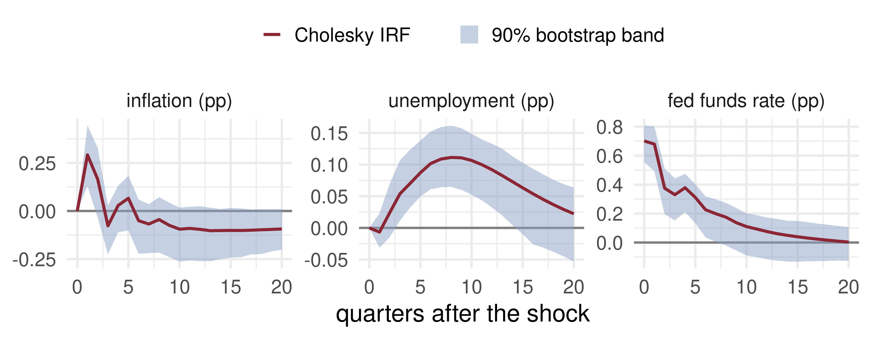
What the data say: after a one-s.d. rate shock the rate decays over about two years and unemployment rises, peaking after two years, as theory predicts. Inflation rises at first and turns negative only after six quarters: the “price puzzle”. A three-variable Cholesky VAR omits information the Fed reacted to (commodity prices, expectations), so part of the “shock” anticipates inflation.

💰 Case Study: Variance Decomposition

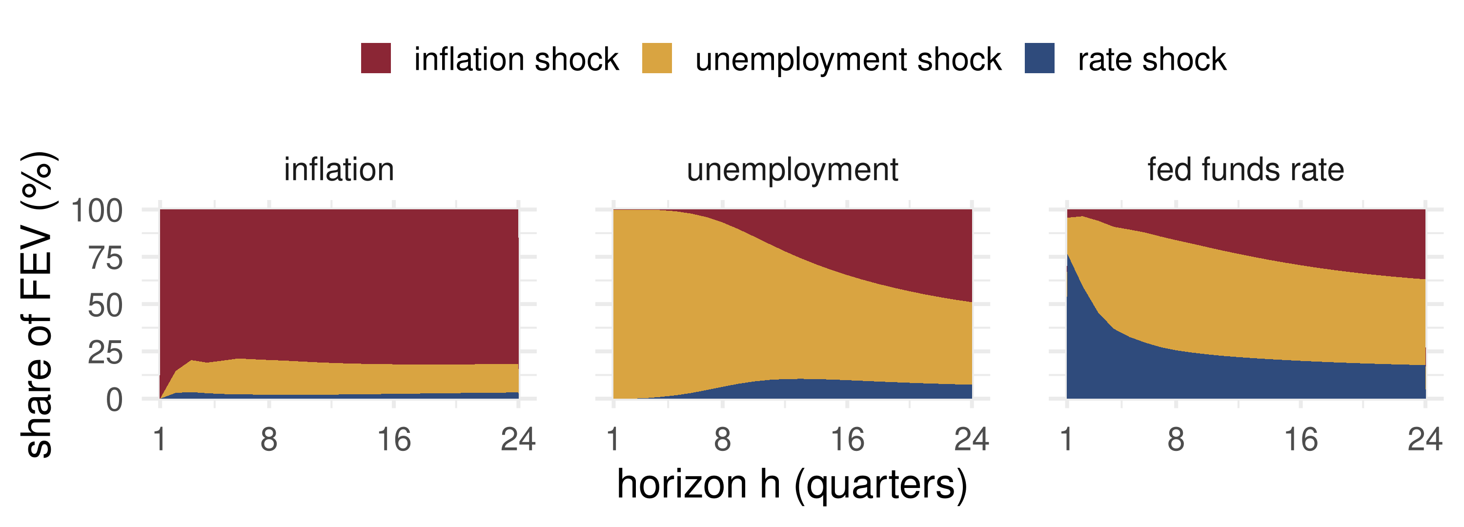
Each panel stacks \(\omega_{ij}(h)\) over the three shocks to 100%. Inflation is driven mostly by its own shock; beyond a year, unemployment shocks carry the largest share of the rate’s forecast errors: the systematic reaction of policy to the real economy.

📝 Quiz #1: Granger Causality

In a bivariate VAR(2) for \((y_t,z_t)\), which restriction says \(z\) does not Granger-cause \(y\)?

The coefficients on \(z_{t-1}\) and \(z_{t-2}\) in the \(y\) equation are both zero
The coefficients on \(y_{t-1}\) and \(y_{t-2}\) in the \(z\) equation are both zero
The correlation between the two innovations is zero
The impact response of \(y\) to the \(z\) shock is zero

📝 Quiz #2: Variance Decomposition

For variable \(j\) at horizon \(h\), \(f_{1j}(h)\sigma_1^2=3\) and \(f_{2j}(h)\sigma_2^2=1\). What is the share of shock 2 in its forecast error variance?

\(25\%\)
\(33\%\)
\(75\%\)
\(1\%\)

📝 Quiz #3: Spurious or Not?

\(x_t\) and \(y_t\) are independent random walks, \(T=1000\). You regress \(y_t\) on \(x_t\) in levels. What do you expect?

A large \(|t|\)-statistic and a sizeable \(R^2\), although there is no relation
A \(t\)-statistic close to \(N(0,1)\), rejecting about 5% of the time
\(R^2\) close to zero, since the series are independent
A cointegrating regression with \(\beta=0\)

📋 Key Formulas

VAR(\(p\))	\(x_t=a_0+\sum_{j=1}^pA_jx_{t-j}+\varepsilon_t\), \(\operatorname{var}\varepsilon_t=\Sigma\)
Stationarity	\(\det(I_m-A_1z-\dots-A_pz^p)\neq0\) for \(\lvert z\rvert\le1\)
Lag choice	\(\text{BIC}(p)=\log\det\hat\Sigma_p+pm^2\log T/T\)
Orthogonal shocks	\(\Sigma=LDL'\), \(v_t=L^{-1}\varepsilon_t\), \(\Psi_s=\Phi_sL\)
IRF	\(\mathrm{IRF}(h)=\partial x_{t+h}/\partial v_t'=\Psi_h\)
FEVD	\(\omega_{ij}(h)=f_{ij}(h)\sigma_i^2/\sum_kf_{kj}(h)\sigma_k^2\), \(f_{ij}(h)=\sum_{s<h}(\Psi_s)_{ji}^2\)
Cointegration	\(x_t,y_t\sim I(1)\), \(y_t-\beta x_t\sim I(0)\)

📋 Summary

A VAR regresses every variable on lags of all of them; OLS equation by equation is efficient
Correlated innovations must be orthogonalised before shocks can be traced; Cholesky ordering is an identifying assumption
IRFs show how a shock propagates; the FEVD says which shocks matter at each horizon
Granger causality is predictive content, not economic causation
Two unrelated \(I(1)\) series regress spuriously; cointegrated series share a stationary combination

📚 Further Reading

Hamilton, J. D. (1994). Time Series Analysis, ch. 10–11 and 18–19; Lütkepohl, H. (2005). New Introduction to Multiple Time Series Analysis, ch. 2–4.
Sims, C. A. (1980). Macroeconomics and reality. Econometrica 48, 1–48.
Granger, C. W. J. (1969). Investigating causal relations by econometric models and cross-spectral methods. Econometrica 37, 424–438.
Granger, C. W. J. and Newbold, P. (1974). Spurious regressions in econometrics. Journal of Econometrics 2, 111–120.
Engle, R. F. and Granger, C. W. J. (1987). Co-integration and error correction. Econometrica 55, 251–276.
Stock, J. H. and Watson, M. W. (2001). Vector autoregressions. Journal of Economic Perspectives 15(4), 101–115.

Next lecture: Volatility: ARCH and GARCH.