Time Series Econometrics

Lecture 15: Volatility — ARCH and GARCH

Samir Orujov, PhD

Open lecture notes, after Stanislav Anatolyev’s course (2016)

🎬 The Idea in 3 Minutes

⬅ Previous lecture: 14 · Vector Autoregressions, Impulse Responses and Cointegration

A short film with the intuition. Watch it before the slides, or after. Captions: CC button.

🎯 Learning Objectives

By the end of this lecture, you will be able to:

• Write the GARCH(1,1) model and derive its unconditional variance, persistence and kurtosis
• Estimate a GARCH(1,1) by Gaussian (quasi-)maximum likelihood with optim()
• Explain why QMLE needs Bollerslev–Wooldridge standard errors
• Test for ARCH effects with the \(TR^2\) Lagrange multiplier statistic
• Recognise the multivariate (BEKK, CCC, DCC), jump and stochastic-volatility extensions

🔁 Warm-up from last time

In a bivariate VAR for \((\Delta m_t, \Delta p_t)\), what does “\(\Delta m\) does not Granger-cause \(\Delta p\)” mean?

• All coefficients on lagged \(\Delta m\) in the \(\Delta p\) equation are zero
• The impulse response of \(\Delta p\) to a money shock is zero at impact
• Money and prices are not cointegrated
• The share of money shocks in the variance decomposition of \(\Delta p\) is 50%

🗺️ Where We Are

Lecture 14 modelled the conditional mean of a vector: \(E(x_t \mid I_{t-1})\) in a VAR, its impulse responses and its variance decomposition.

Lecture 1 gave a warning we have not yet used. A series can be stationary with a constant unconditional variance while its conditional variance moves over time.

Today the object of interest is that conditional variance, \[\sigma_t^2 = \operatorname{var}(r_t \mid I_{t-1}),\] for a single return series \(r_t\).

❓ The Question

How risky is tomorrow?

A risk desk holds an S&P 500 index position. On a calm day the index moves by about half a percent; in March 2020 it moved by 5–12% a day for weeks.

Returns are nearly unpredictable in mean, so the conditional mean is of little use. Their size is predictable: a large move today makes a large move tomorrow more likely. Margins, Value-at-Risk and option prices all need a forecast of that size.

📈 Volatility Clusters

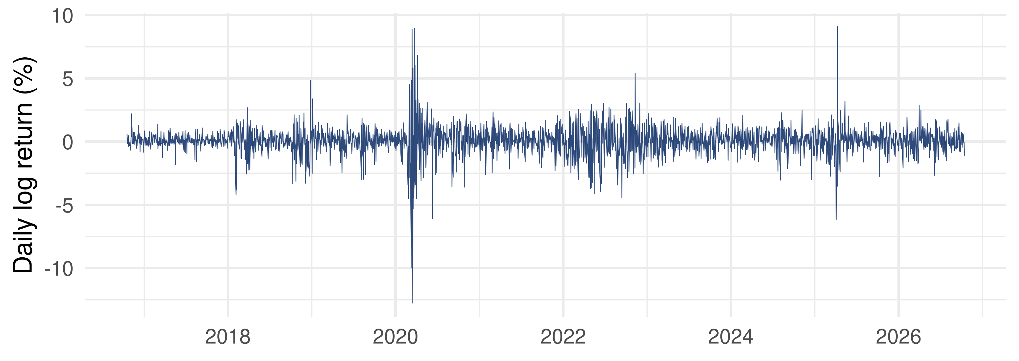
S&P 500, October 2016 – October 2026. Quiet stretches alternate with turbulent ones: large moves of either sign come in clusters.

📐 The GARCH(1,1) Model

GARCH(1,1) (Bollerslev, 1986)

\[r_t = \mu_t + \varepsilon_t, \qquad \varepsilon_t = \sigma_t \eta_t, \qquad \eta_t \sim \text{iid } \mathcal N(0,1),\] \[\sigma_t^2 = \omega + \alpha\,\varepsilon_{t-1}^2 + \beta\,\sigma_{t-1}^2, \qquad \omega > 0,\ \alpha \ge 0,\ \beta \ge 0.\]

• \(\mu_t = E(r_t \mid I_{t-1})\) is the conditional mean: a constant, or an AR term
• \(\sigma_t^2\) is known at \(t-1\): it is the conditional variance of \(r_t\)
• \(\alpha\) is the reaction to yesterday’s news \(\varepsilon_{t-1}^2\); \(\beta\) is the memory of yesterday’s variance
• \(\beta = 0\) gives Engle’s (1982) ARCH(1); ARCH(\(q\)) has \(\sigma_t^2 = \omega + \alpha_1\varepsilon_{t-1}^2 + \dots + \alpha_q\varepsilon_{t-q}^2\)

📐 A Predictive Model: AR-ARCH-M

Lecture 3 used this as the example of a non-structural model, built for fit and forecasting rather than derived from an optimising agent: \[r_t = c + \rho\, r_{t-1} + \delta\,\sigma_t^2 + \varepsilon_t, \qquad \varepsilon_t \mid I_{t-1} \sim (0, \sigma_t^2), \qquad \sigma_t^2 = \omega + \alpha\,\varepsilon_{t-1}^2 .\]

• The variance enters the mean (“in mean”, M): \(\delta\) is the price of risk
• \(\delta > 0\) says investors demand a higher expected return when conditional risk is higher
• Mean and variance must now be estimated jointly; a wrong variance equation also biases \(\hat c\), \(\hat\rho\), \(\hat\delta\)

📐 Properties: Unconditional Variance

Take expectations of the variance equation. Since \(E\varepsilon_{t-1}^2 = E\big[E(\varepsilon_{t-1}^2 \mid I_{t-2})\big] = E\sigma_{t-1}^2\), under stationarity \(E\sigma_t^2 = \bar\sigma^2\) for all \(t\): \[\bar\sigma^2 = \omega + \alpha\bar\sigma^2 + \beta\bar\sigma^2 \quad\Longrightarrow\quad \bar\sigma^2 = \operatorname{var}(\varepsilon_t) = \frac{\omega}{1-\alpha-\beta}.\]

• A finite, positive solution needs \(\alpha + \beta < 1\): this is the condition for covariance stationarity
• \(\varepsilon_t\) is then weak white noise, indeed an MDS: uncorrelated, constant variance \(\bar\sigma^2\), yet not independent
• With \(\alpha + \beta = 1\) (IGARCH) the unconditional variance is infinite

Not in the 2016 notes: added from Bollerslev (1986) and Tsay (2010), ch. 3.

📐 Properties: Persistence and Half-Life

Write \(v_t = \varepsilon_t^2 - \sigma_t^2\), an MDS. Then GARCH(1,1) is an ARMA(1,1) in \(\varepsilon_t^2\): \[\varepsilon_t^2 = \omega + (\alpha+\beta)\,\varepsilon_{t-1}^2 + v_t - \beta\, v_{t-1}.\]

Iterating the variance equation forward gives the \(h\)-step forecast \[\sigma_{t+h \mid t}^2 = \bar\sigma^2 + (\alpha+\beta)^{h-1}\big(\sigma_{t+1}^2 - \bar\sigma^2\big).\]

• \(\alpha + \beta\) is the persistence: the rate at which a variance shock decays
• Half-life: \((\alpha+\beta)^h = \tfrac12\), so \(h_{1/2} = \ln 0.5 / \ln(\alpha+\beta)\)

Not in the 2016 notes: added from Bollerslev (1986) and Tsay (2010), ch. 3.

📐 Properties: Fat Tails

With \(\eta_t \sim \mathcal N(0,1)\), \(E\varepsilon_t^4 = 3E\sigma_t^4 \ge 3(E\sigma_t^2)^2\) by Jensen. A random variance mixes normals, and the mixture has fatter tails. For GARCH(1,1) the kurtosis is \[\kappa = \frac{E\varepsilon_t^4}{(E\varepsilon_t^2)^2} = \frac{3\big[1-(\alpha+\beta)^2\big]}{1-(\alpha+\beta)^2-2\alpha^2} > 3,\] finite only if \((\alpha+\beta)^2 + 2\alpha^2 < 1\). For ARCH(1): \(\kappa = 3(1-\alpha^2)/(1-3\alpha^2)\), finite if \(\alpha^2 < 1/3\).

Volatility clustering and fat tails are one phenomenon, not two.

Not in the 2016 notes: added from Bollerslev (1986) and Tsay (2010), ch. 3.

✏️ Worked Example: A GARCH Forecast

Daily returns in %: \(\omega = 0.02\), \(\alpha = 0.08\), \(\beta = 0.90\). Today \(\sigma_t^2 = 1.5\) and the shock was \(\varepsilon_t = -3\).

1. Long-run level. \(\bar\sigma^2 = 0.02/(1-0.98) = 1\): daily sd 1%, annualised \(1\% \times \sqrt{252} = 15.9\%\).

2. Tomorrow. \(\sigma_{t+1}^2 = 0.02 + 0.08 \cdot 9 + 0.90 \cdot 1.5 = 2.09\): daily sd 1.45%.

3. Ten days ahead. \(\sigma_{t+10 \mid t}^2 = 1 + 0.98^{9}(2.09 - 1) = 1 + 0.834 \cdot 1.09 = 1.91\).

4. Half-life \(= \ln 0.5/\ln 0.98 = 34.3\) days. Kurtosis \(= 3(1-0.9604)/(1-0.9604-0.0128) = 0.1188/0.0268 = 4.43\).

📐 Estimation: Gaussian MLE

With \(\theta = (\text{parameters of } \mu_t,\ \omega,\ \alpha,\ \beta)\) and, up to a constant, \[\ell_t(\theta) = -\tfrac12 \log\sigma_t^2 - \frac{(r_t-\mu_t)^2}{2\sigma_t^2},\] \[\hat\theta = \arg\max_\theta \sum_{t=1}^T \ell_t(\theta) \quad \text{s.t.} \quad \sigma_t^2 = \omega + \alpha\varepsilon_{t-1}^2 + \beta\sigma_{t-1}^2 .\]

• \(\sigma_t^2\) is computed recursively, so it needs a start value \(\sigma_1^2\): \(\ \omega/(1-\alpha-\beta)\), or the sample variance \(\frac1T\sum(r_t-\bar r)^2\), or an extra parameter
• Restrictions \(\omega > 0\), \(\alpha, \beta \ge 0\) keep every \(\sigma_t^2\) positive

📐 Asymptotics of the MLE

If the model, including normality of \(\eta_t\), is correct: \[\hat\theta \xrightarrow{p} \theta, \qquad \sqrt T(\hat\theta-\theta) \xrightarrow{d} \mathcal N\big(0,\ I^{-1}\big),\] \[I = E\!\left[\frac{\partial \ell_t}{\partial\theta}\frac{\partial \ell_t}{\partial\theta'}\right] = -E\!\left[\frac{\partial^2 \ell_t}{\partial\theta\,\partial\theta'}\right].\]

The second equality is the information matrix equality. It holds because the likelihood is the true density. It is the first thing to fail when the density is wrong.

📐 When \(\eta_t\) Is Not Normal

• A known family. If \(\eta_t \sim \text{iid } \mathcal D(0,1,\varphi)\), e.g. a Student-\(t\) normalised to mean 0 and variance 1, then \(\varphi\) joins \(\theta\) and \(\ell_t = \log f_{\mathcal D}\). Run MLE based on \(\mathcal D\).
• ARCD (autoregressive conditional density): let the shape parameters \(\varphi\) themselves move over time.
• Nothing specified. Keep the Gaussian likelihood anyway: this is quasi-MLE (QMLE). The optimisation is the same; the asymptotics change.

If the distribution is wrong, a non-Gaussian MLE (say Student-\(t\) when the truth is not \(t\)) is in general inconsistent. The Gaussian QMLE stays consistent provided the conditional mean and variance are correctly specified.

📐 QMLE: The Sandwich

Gaussian QMLE (Bollerslev & Wooldridge, 1992)

\[\hat\theta \xrightarrow{p} \theta, \qquad \sqrt T(\hat\theta-\theta) \xrightarrow{d} \mathcal N\big(0,\ J^{-1} I J^{-1}\big),\] \[J = -E\!\left[\frac{\partial^2 \ell_t}{\partial\theta\,\partial\theta'}\right], \qquad I = E\!\left[\frac{\partial \ell_t}{\partial\theta}\frac{\partial \ell_t}{\partial\theta'}\right].\]

• Under non-normal \(\eta_t\), \(I \neq J\), so \(J^{-1}\) alone is the wrong variance
• Bollerslev–Wooldridge robust standard errors: estimate \(J\) by the average Hessian and \(I\) by the average outer product of the scores, both at \(\hat\theta\)

💻 The Quasi-Likelihood in R

# theta = (mu, omega, alpha, beta); returns r in percent
sig2_path <- function(th, r) {                 # the variance recursion
  e <- r - th[1]; s2 <- numeric(length(r)); s2[1] <- var(r)   # start value
  for (t in 2:length(r)) s2[t] <- th[2] + th[3] * e[t-1]^2 + th[4] * s2[t-1]
  s2
}
ell <- function(th, r) {                       # the vector of l_t(theta)
  s2 <- sig2_path(th, r); -0.5 * log(s2) - (r - th[1])^2 / (2 * s2)
}
nll <- function(th, r) {                       # minus the quasi-log-likelihood
  if (th[2] <= 0 || th[3] < 0 || th[4] < 0 || th[3] + th[4] >= 1) return(1e10)
  -sum(ell(th, r))
}

The restrictions enter as a wall: outside the parameter space the objective is \(10^{10}\), so optim() never steps there. The start value is the sample variance.

💻 Does It Recover the Truth?

qmle <- function(r, start = c(mean(r), 0.05, 0.10, 0.85)) {
  f  <- optim(start, nll, r = r, control = list(maxit = 5000, reltol = 1e-12))
  f  <- optim(f$par, nll, r = r, method = "BFGS", control = list(reltol = 1e-12))
  th <- f$par
  H  <- optimHess(th, nll, r = r)                       # numerical T * J-hat
  S  <- sapply(1:4, function(k) { h <- rep(0, 4); h[k] <- 1e-5
          (ell(th + h, r) - ell(th - h, r)) / 2e-5 })    # T x 4 numerical scores
  Hi <- solve(H)
  out <- list(theta = th, se_hess = sqrt(diag(Hi)),
              se_bw = sqrt(diag(Hi %*% crossprod(S) %*% Hi)))
  lapply(out, setNames, c("mu", "omega", "alpha", "beta"))
}
set.seed(2026)
n <- 3000; th0 <- c(0.05, 0.05, 0.10, 0.85)
eta <- rt(n, df = 5) / sqrt(5 / 3)            # Student-t(5), scaled to variance 1
r_sim <- numeric(n); s2 <- th0[2] / (1 - th0[3] - th0[4]); e_prev <- 0
for (t in 1:n) {
  s2 <- th0[2] + th0[3] * e_prev^2 + th0[4] * s2
  e_prev <- sqrt(s2) * eta[t]; r_sim[t] <- th0[1] + e_prev
}
fit_sim <- qmle(r_sim)
round(rbind(truth = th0, estimate = fit_sim$theta,
            se_Hessian = fit_sim$se_hess, se_BW = fit_sim$se_bw), 4)

               mu  omega  alpha   beta
truth      0.0500 0.0500 0.1000 0.8500
estimate   0.0578 0.0476 0.0977 0.8440
se_Hessian 0.0145 0.0084 0.0125 0.0186
se_BW      0.0147 0.0122 0.0173 0.0247

The shocks are Student-\(t\), so this is QMLE. The estimates sit near the truth; the robust (BW) errors on \(\omega, \alpha, \beta\) exceed the inverse-Hessian ones by a third to a half. Both use numerical derivatives.

🧪 Testing for ARCH Effects

In ARCH(\(q\)), \(\sigma_t^2 = \omega + \alpha_1\varepsilon_{t-1}^2 + \dots + \alpha_q\varepsilon_{t-q}^2\) with \(\alpha_i \ge 0\), test \[H_0:\ \alpha_1 = \dots = \alpha_q = 0 .\]

All other tests in GARCH models are standard; this one is not. Under \(H_0\) the parameters sit on the boundary \(\alpha_i = 0\), and in a GARCH alternative \(\beta\) is not even identified.

Engle’s LM test

Regress \(\hat\varepsilon_t^2\) on a constant and \(\hat\varepsilon_{t-1}^2, \dots, \hat\varepsilon_{t-q}^2\) (\(\hat\varepsilon_t\): OLS residuals of the mean equation). Then \[LM = T R^2 \xrightarrow[H_0]{d} \chi^2_q .\]

Only the model under \(H_0\) is estimated, so the boundary does no harm.

🧠 Think-Pair-Share

A colleague fits a GARCH(1,1) to daily returns in % and reports \[\hat\omega = 0.03, \qquad \hat\alpha = 0.15, \qquad \hat\beta = 0.83 .\]

1. What is the half-life of a volatility shock?
2. What annualised volatility does the model revert to?
3. Does the fitted model have a finite fourth moment?

✅ Think-Pair-Share: Solution

1. Persistence \(\hat\alpha + \hat\beta = 0.98\), so \(h_{1/2} = \ln 0.5/\ln 0.98 = 34.3\) trading days, about seven weeks.

2. \(\bar\sigma^2 = 0.03/0.02 = 1.5\), a daily sd of \(1.22\%\), annualised \(1.22\sqrt{252} = 19.4\%\).

3. \((\hat\alpha+\hat\beta)^2 + 2\hat\alpha^2 = 0.9604 + 0.045 = 1.005 > 1\). No: the fourth moment is infinite.

Same persistence as the worked example, but a larger \(\alpha\): a twice as violent reaction to news. That alone is enough to destroy the fourth moment, and with it the usual interpretation of a sample kurtosis.

🎛️ Explore: \(\alpha\), \(\beta\) and Clustering

viewof alpha = {
  const input = Inputs.range([0, 0.4], {value: 0.10, step: 0.01, label: "α (news)"});
  ['pointerdown','touchstart','mousedown','click','wheel','pointermove','touchmove']
    .forEach(e => input.addEventListener(e, ev => ev.stopPropagation()));
  return input;
}
viewof beta = {
  const input = Inputs.range([0, 0.95], {value: 0.88, step: 0.01, label: "β (memory)"});
  ['pointerdown','touchstart','mousedown','click','wheel','pointermove','touchmove']
    .forEach(e => input.addEventListener(e, ev => ev.stopPropagation()));
  return input;
}

shocks = {
  let s = 20261;
  const u = () => (s = (s * 1103515245 + 12345) % 2147483648) / 2147483648;
  return Array.from({length: 1000}, () =>
    Math.sqrt(-2 * Math.log(Math.max(u(), 1e-12))) * Math.cos(2 * Math.PI * u()));
}
path = {
  const p = alpha + beta, omega = p < 1 ? 1 - p : 0.01;   // long-run variance 1 when p < 1
  let s2 = 1, e = 0; const out = [];
  for (let t = 0; t < shocks.length; t++) {
    s2 = omega + alpha * e * e + beta * s2;
    e = Math.sqrt(s2) * shocks[t];
    out.push({t: t + 1, r: e, sd: Math.sqrt(s2)});
  }
  return out;
}

Plot.plot({
  width: 1100, height: 300, marginLeft: 70, marginBottom: 50,
  style: {fontSize: "18px"},
  x: {label: "day"}, y: {label: "return", grid: true},
  marks: [
    Plot.ruleY([0]),
    Plot.lineY(path, {x: "t", y: "r", stroke: "#8ba3c7", strokeWidth: 1}),
    Plot.lineY(path, {x: "t", y: d => 2 * d.sd, stroke: "#8b2635", strokeWidth: 2}),
    Plot.lineY(path, {x: "t", y: d => -2 * d.sd, stroke: "#8b2635", strokeWidth: 2})
  ]
})

html`<div style="font-size:28px">α + β = ${(alpha + beta).toFixed(2)} ${alpha + beta < 1
  ? `· half-life ${(Math.log(0.5) / Math.log(alpha + beta)).toFixed(1)} days`
  : "· not covariance stationary"} · red: ±2σ<sub>t</sub>, same shocks throughout</div>`

🌐 Multivariate GARCH: VECH and BEKK

For \(m\) assets, \(r_t = \varepsilon_t \mid I_{t-1} \sim (0, \Omega_t)\) with \(\Omega_t\) an \(m\times m\) conditional covariance matrix.

VECH. With \(\operatorname{vech}\) stacking the elements on and below the diagonal: \[\operatorname{vech}(\Omega_t) = \operatorname{vech}(\Sigma) + A\operatorname{vech}(\varepsilon_{t-1}\varepsilon_{t-1}') + B\operatorname{vech}(\Omega_{t-1}),\] \(A, B\) of size \(\tfrac{m(m+1)}{2}\times\tfrac{m(m+1)}{2}\). Too many parameters, and \(\Omega_t\) need not be positive definite.

BEKK (Baba, Engle, Kraft, Kroner): \[\Omega_t = \Sigma + A\,\varepsilon_{t-1}\varepsilon_{t-1}'A' + B\,\Omega_{t-1}B', \qquad A, B \ \ m\times m .\] More parsimonious, and positive definite by construction when \(\Sigma\) is.

🌐 Multivariate GARCH: CCC and DCC

CCC (constant conditional correlations, Bollerslev 1990): \[\Omega_t = C_t R\, C_t, \qquad C_t = \operatorname{diag}(\sigma_{1t}, \dots, \sigma_{mt}), \qquad \sigma_{it}^2 = \omega_i + \alpha_i\varepsilon_{i,t-1}^2 + \beta_i\sigma_{i,t-1}^2,\] with \(R\) a constant correlation matrix. Each asset gets its own GARCH.

DCC (dynamic conditional correlations, Engle 2002). In real data correlations are not constant, so let \(R_t\) move: \[\Omega_t = C_t R_t C_t, \qquad (R_t)_{ij} = \frac{q_{ijt}}{\sqrt{q_{iit}\,q_{jjt}}},\] \[q_{ijt} = \bar q_{ij}(1-\alpha-\beta) + \alpha\, z_{i,t-1}z_{j,t-1} + \beta\, q_{ij,t-1}, \qquad z_{it} = \varepsilon_{it}/\sigma_{it},\] with one pair \((\alpha, \beta)\) common to all \(i, j\).

⚡ ARCH with Jumps; Stochastic Volatility

ARCH with jumps. Within a day the price sometimes jumps. For daily returns, \[r_t = \mu + \varepsilon_t + \sum_{j=1}^{N_t} g_{jt}, \qquad \varepsilon_t \sim \text{GARCH}(1,1), \qquad g_{jt} \sim \text{iid } \mathcal N(\theta, \delta^2),\] with \(N_t \sim \text{Poisson}(\lambda_t)\) jumps on day \(t\); the intensity \(\lambda_t\) follows ARMA-type dynamics.

Stochastic volatility. \[\varepsilon_t = \sigma_t\eta_t, \qquad \log\sigma_t^2 = \omega + \beta\log\sigma_{t-1}^2 + v_t, \qquad v_t \sim \text{iid } \mathcal N(0, \sigma_v^2) \perp \eta_t .\] The variance has its own shock \(v_t\), which makes SV more flexible than GARCH. The price: \(\sigma_t^2\) is latent, so the likelihood has no closed form and needs filtering or simulation.

💰 Case Study: S&P 500 Volatility

📈 The question

A risk desk wants a daily volatility model for the index.

1. Are there ARCH effects at all?
2. How persistent is volatility, and where does it revert to?
3. Do robust and Hessian standard errors differ?

📊 The data

Series: S&P 500 close, FRED SP500

Period: 18 Oct 2016 – 14 Oct 2026, 2,511 trading days

Transformation: \(r_t = 100\,\Delta\log P_t\), daily log returns in %; \(\mu_t = \mu\) constant

sp <- read.csv("https://fred.stlouisfed.org/graph/fredgraph.csv?id=SP500")

💰 Case Study: QMLE and the LM Test

r <- r_all; n_r <- length(r)
e2 <- (r - mean(r))^2; X <- embed(e2, 6)                 # e2_t and 5 lags
LM <- nrow(X) * summary(lm(X[, 1] ~ X[, -1]))$r.squared
fit <- qmle(r); th <- fit$theta; p <- unname(th[3] + th[4])
z <- (r - th[1]) / sqrt(sig2_path(th, r))
kurt <- function(x) mean((x - mean(x))^4) / mean((x - mean(x))^2)^2
list(ARCH_LM = signif(c(LM = LM, p_value = pchisq(LM, 5, lower.tail = FALSE)), 3),
     estimates = round(rbind(theta = th, se_Hessian = fit$se_hess,
                             se_BW = fit$se_bw), 4),
     implied = round(c(persistence = p, half_life_days = log(0.5) / log(p),
                       annual_vol = unname(sqrt(252 * th[2] / (1 - p))),
                       kurt_r = kurt(r), kurt_eta_hat = kurt(z)), 3))

$ARCH_LM
       LM   p_value 
 7.68e+02 9.59e-164 

$estimates
               mu  omega  alpha   beta
theta      0.0854 0.0340 0.1603 0.8131
se_Hessian 0.0147 0.0058 0.0184 0.0188
se_BW      0.0150 0.0101 0.0271 0.0287

$implied
   persistence half_life_days     annual_vol         kurt_r   kurt_eta_hat 
         0.973         25.662         17.924         19.753          5.530 

Look at \(LM\), the persistence, and the two rows of standard errors.

💰 Case Study: Fitted Volatility

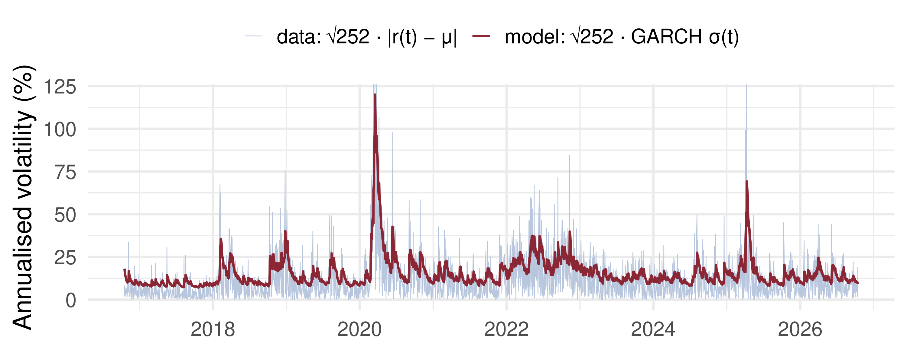
What the data say: the LM test rejects no ARCH emphatically, and \(\hat\alpha + \hat\beta \approx 0.97\): volatility shocks halve in about a month, and \(\sigma_t\) tracks every cluster. The model does not remove the fat tails: the standardised residuals still have kurtosis near 5.5, not 3, which is why the robust errors on \(\omega, \alpha, \beta\) run 50–75% above the Hessian ones.

📉 The News-Impact Curve

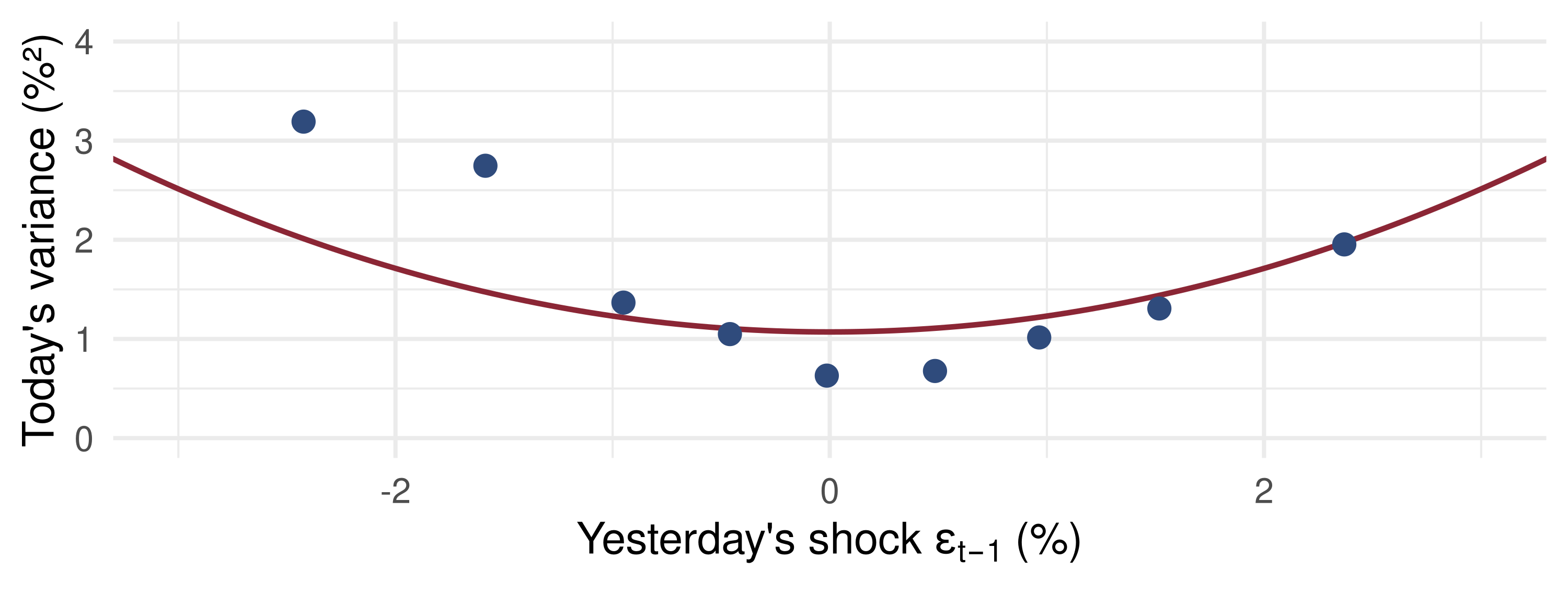
Red: \(\sigma_t^2 = \hat\omega + \hat\alpha\varepsilon_{t-1}^2 + \hat\beta\bar\sigma^2\), a parabola symmetric in the news. Blue: average realised \(\varepsilon_t^2\) in bins of \(\varepsilon_{t-1}\), symmetric about 0. Falls are followed by more volatility than rises of equal size (the leverage effect), which a symmetric GARCH cannot produce.

📝 Quiz #1: Stationarity

A GARCH(1,1) has \(\omega = 0.04\), \(\alpha = 0.06\), \(\beta = 0.90\). What is the unconditional variance of \(\varepsilon_t\)?

• \(1.0\)
• \(0.04\)
• \(0.4\)
• It does not exist, since \(\beta\) is close to 1

📝 Quiz #2: Robust Errors

You estimate a GARCH by the Gaussian likelihood, but the standardised residuals have kurtosis 5. What should you report?

• The estimates as they are, with sandwich \(J^{-1}IJ^{-1}\) (Bollerslev–Wooldridge) standard errors
• The inverse-Hessian standard errors, since the MLE is efficient
• Nothing: the estimates are inconsistent and must be discarded
• Standard errors from a Student-\(t\) likelihood fitted to the same estimates

📝 Quiz #3: The ARCH-LM Test

With \(T = 1000\) and \(q = 4\), the regression of \(\hat\varepsilon_t^2\) on four of its lags has \(R^2 = 0.012\). At 5% (\(\chi^2_4\) critical value 9.49):

• \(LM = 12 > 9.49\): reject “no ARCH effects”
• \(LM = 0.012\): do not reject
• \(LM = 3\): do not reject
• The test is invalid, because \(\alpha_i = 0\) lies on the boundary

📋 Key Formulas

GARCH(1,1)	\(\sigma_t^2 = \omega + \alpha\varepsilon_{t-1}^2 + \beta\sigma_{t-1}^2\), \(\ \varepsilon_t = \sigma_t\eta_t\)
Unconditional variance	\(\bar\sigma^2 = \omega/(1-\alpha-\beta)\), needs \(\alpha+\beta<1\)
Forecast, half-life	\(\sigma^2_{t+h\mid t} = \bar\sigma^2 + (\alpha+\beta)^{h-1}(\sigma^2_{t+1}-\bar\sigma^2)\), \(\ h_{1/2} = \frac{\ln 0.5}{\ln(\alpha+\beta)}\)
Kurtosis (normal \(\eta_t\))	\(3[1-(\alpha+\beta)^2]/[1-(\alpha+\beta)^2-2\alpha^2]\)
Gaussian \(\ell_t\)	\(-\frac12\log\sigma_t^2 - (r_t-\mu_t)^2/(2\sigma_t^2)\)
MLE / QMLE	\(\mathcal N(0, I^{-1})\) / \(\mathcal N(0, J^{-1}IJ^{-1})\)
ARCH-LM	\(TR^2 \to \chi^2_q\)

📋 Summary

• GARCH models the conditional variance; \(\varepsilon_t\) stays white noise but is not independent
• \(\alpha + \beta\) is the persistence; \(\alpha + \beta < 1\) gives a finite unconditional variance
• Random variance plus normal shocks gives fat tails: clustering and kurtosis are one fact
• Estimate by Gaussian (Q)MLE; under non-normal shocks keep the estimates and use Bollerslev–Wooldridge errors
• Test for ARCH with \(TR^2\); the boundary makes Wald and LR non-standard
• BEKK, CCC and DCC extend GARCH to many assets; jumps and SV add a second source of randomness

📚 Further Reading

• Engle (1982), Econometrica: ARCH and the LM test
• Bollerslev (1986), J. Econometrics: GARCH; Bollerslev & Wooldridge (1992), Econometric Reviews: QMLE
• Engle, Lilien & Robins (1987), Econometrica: ARCH-M
• Engle & Kroner (1995), Bollerslev (1990), Engle (2002): BEKK, CCC, DCC
• Hamilton (1994), ch. 21; Tsay (2010), ch. 3 and 10; Francq & Zakoïan (2019), GARCH Models

Next lecture: 16 · Structural Breaks and Parameter Stability