Time Series Econometrics

Lecture 16: Structural Breaks and Parameter Stability

Samir Orujov, PhD

Open lecture notes, after Stanislav Anatolyev’s course (2016)

🎬 The Idea in 2 Minutes

⬅ Previous lecture: 15 · Volatility — ARCH and GARCH

A short film with the intuition. Watch it before the slides, or after. Captions: CC button.

🎯 Learning Objectives

By the end of this lecture, you will be able to:

  • Test for a break at a known date with a Wald statistic, and at an unknown date with Andrews’ sup-Wald
  • Explain why searching over dates changes the critical value, and why the search is trimmed
  • Estimate several break dates by Bai–Perron least squares and choose their number sequentially
  • Construct the CUSUM test from recursive residuals and read it against its boundaries
  • Locate the breaks in the mean of US inflation

🔁 Warm-up from last time

A GARCH(1,1) for daily returns has \(\alpha + \beta = 0.95\). After a volatility shock, roughly how many days until half of the excess variance has gone?

  • About 13.5 days
  • About 0.95 days
  • About 20 days, one trading month
  • Never: with \(\alpha + \beta\) near 1 the variance is infinite

🗺️ Where We Are

Lecture 15 fitted one GARCH with one set of parameters \((\omega, \alpha, \beta)\) to ten years of returns. Every model in this course has made the same assumption: the parameters do not change over the sample.

Lectures 11–12 let the parameters switch with the value of a threshold variable \(q_t \lessgtr \gamma\).

Today the switching variable is time itself: the parameters change at a date \(T_1\). Is there such a date? Where is it? Are there several?

❓ The Question

Did inflation change regime?

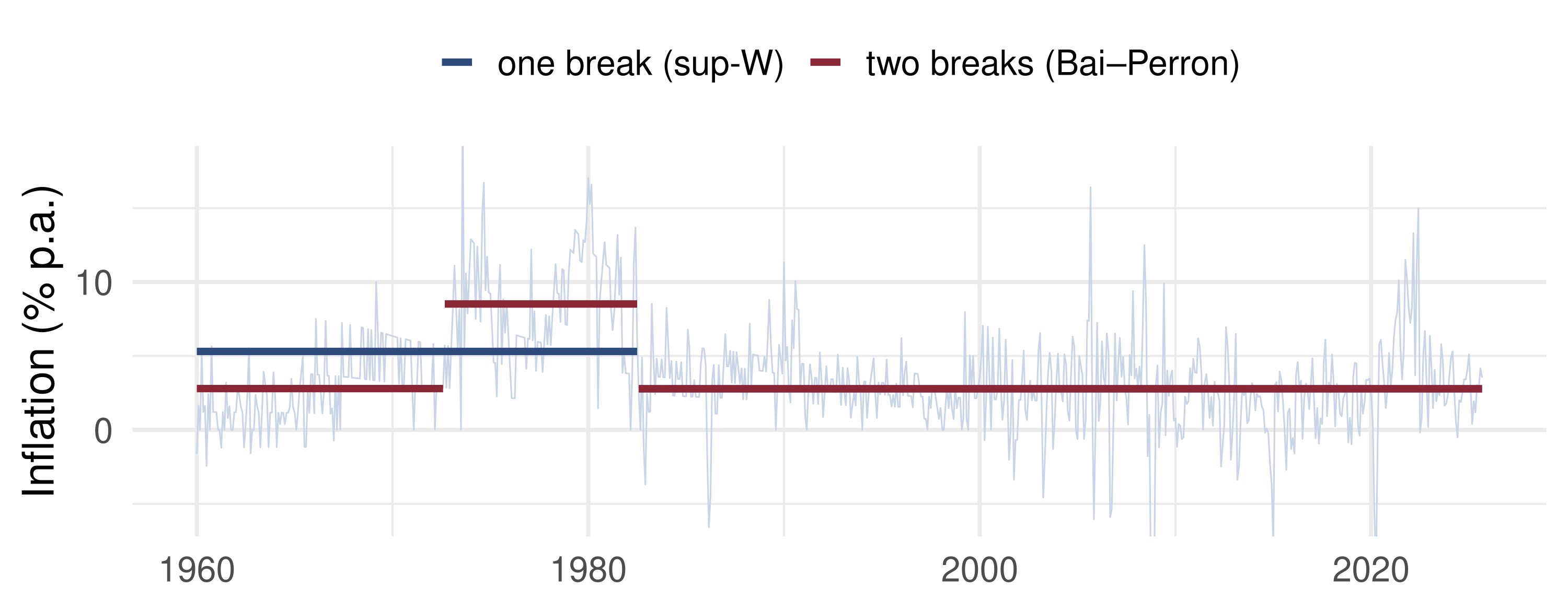
US CPI inflation averaged under 3% in the early 1960s, near 9% in the 1970s and under 3% after the Volcker disinflation of 1979–1982.

A forecaster who uses the full-sample mean is averaging over regimes that no longer exist. Before choosing a sample, one must ask whether the mean is stable, and if not, when it moved. The date is not given in advance: it must be found from the data.

📐 One Break: The Model

With \(x_t \in \mathbb R^k\) and a candidate break date \(T_1\), \[y_t = x_t'\beta + x_t'\delta\,\mathbb 1\{t > T_1\} + e_t, \qquad t = 1, \dots, T .\]

  • Before \(T_1\) the coefficients are \(\beta\), after it \(\beta + \delta\)
  • No break: \(H_0: \delta = 0\), a set of \(k\) linear restrictions
  • The simplest case, \(x_t = 1\), is a break in the mean: \(\mu_1\) before \(T_1\), \(\mu_2 = \mu_1 + \delta\) after

Known date (Chow): the Wald statistic satisfies \[W(T_1) \xrightarrow[H_0]{d} \chi^2_k .\]

📐 An Unknown Date: sup-Wald

If \(T_1\) is unknown, compute \(W(T_1)\) at every admissible date and take the largest: \[\sup W = \max_{\pi T \le T_1 \le (1-\pi)T} W(T_1) \xrightarrow[H_0]{d} \sup_{\pi \le r \le 1-\pi} Q(r), \qquad Q(r) = \frac{\|B(r) - rB(1)\|^2}{r(1-r)},\] with \(B\) a \(k\)-dimensional standard Brownian motion (Andrews, 1993, 2003).

  • The maximum of many \(\chi^2\)-like statistics is not \(\chi^2\): the critical values are larger
  • They depend on \(k\) and on the trimming \(\pi\): how far from the endpoints a break may lie
  • For \(k = 1\), \(\pi = 0.15\): the 5% critical value is \(8.68\), not \(3.84\)

📐 Why Trim?

\(B(r) - rB(1)\) is a Brownian bridge, with variance \(r(1-r)\). So for each fixed \(r\), \(Q(r) \sim \chi^2_k\): the known-date result.

Near the ends, \(r(1-r) \to 0\) and the bridge is divided by almost nothing. By the law of the iterated logarithm, \[\sup_{0 < r < 1} Q(r) = \infty \quad \text{almost surely.}\]

Without trimming, a test would find a “break” in the first or last few observations of every series. With \(\pi = 0.15\) the search runs over the middle 70% of the sample. A smaller \(\pi\) searches more dates and needs a larger critical value.

✏️ Worked Example: A Searched Date

\(T = 100\) quarterly growth rates. Splitting at \(T_1 = 40\) gives means \(\bar y_1 = 2.0\) and \(\bar y_2 = 3.0\); the pooled residual variance is \(\hat\sigma^2 = 4\).

Wald statistic. \(\widehat{\operatorname{var}}(\bar y_2 - \bar y_1) = \hat\sigma^2\big(\tfrac1{40} + \tfrac1{60}\big) = 4 \times 0.04167 = 0.1667\), so \[W(40) = \frac{(3.0 - 2.0)^2}{0.1667} = 6.0 .\]

If 40 was fixed in advance (a policy change in quarter 40): \(6.0 > 3.84 = \chi^2_{1, 0.95}\). Reject: there is a break.

If 40 was the date that maximised \(W\): \(6.0 < 8.68\). Do not reject. The same number is weaker evidence once it has been searched for.

💻 sup-Wald in R

wald_path <- function(y, trim = 0.15) {      # W(T1) for a break in the mean
  n <- length(y); cs <- cumsum(y); W <- rep(NA_real_, n)
  for (T1 in ceiling(trim * n):floor((1 - trim) * n)) {
    m1 <- cs[T1] / T1; m2 <- (cs[n] - cs[T1]) / (n - T1)
    rss <- sum((y[1:T1] - m1)^2) + sum((y[(T1 + 1):n] - m2)^2)
    W[T1] <- (m2 - m1)^2 / (rss / (n - 2) * (1 / T1 + 1 / (n - T1)))
  }
  W
}
set.seed(2026)
y0 <- rnorm(200); y1 <- rnorm(200) + 0.6 * (seq_len(200) > 120)  # break at 120
round(c(supW_no_break = max(wald_path(y0), na.rm = TRUE),
        supW_break = max(wald_path(y1), na.rm = TRUE),
        argmax_break = which.max(wald_path(y1))), 2)
supW_no_break    supW_break  argmax_break 
         5.72         15.17        118.00 
Without a break the maximum stays below 8.68; with one it is far above, and the arg max lands near \(t = 120\).

💻 Where Does 8.68 Come From?

📦 Simulate sup Q(r) for k = 1 at three trimmings
set.seed(2026)
n_grid <- 2000; reps <- 3000; r <- (1:n_grid) / n_grid
sup_Q <- function(trim) replicate(reps, {
  B <- cumsum(rnorm(n_grid)) / sqrt(n_grid)
  bridge <- B - r * B[n_grid]
  keep <- r >= trim & r <= 1 - trim
  max(bridge[keep]^2 / (r[keep] * (1 - r[keep])))
})
crit <- sapply(c(0.05, 0.15, 0.30), function(p) quantile(sup_Q(p), 0.95))
names(crit) <- c("trim 0.05", "trim 0.15", "trim 0.30")
round(c(chi2_1 = qchisq(0.95, 1), crit), 2)
   chi2_1 trim 0.05 trim 0.15 trim 0.30 
     3.84      9.82      8.31      7.24 

The simulated 5% value at \(\pi = 0.15\) is close to Andrews’ 8.68 (a finite grid slightly understates the supremum). Wider searches demand larger values; every one exceeds \(3.84\).

📐 Many Breaks: Bai & Perron (1998)

Now \(m\) breaks, \(m\) known, so \(m+1\) stable regimes: \[y_t = x_t'\beta_j + e_t, \qquad t = T_{j-1}+1, \dots, T_j, \quad j = 1, \dots, m+1, \quad T_0 = 0,\ T_{m+1} = T .\]

Estimate everything by least squares, with a minimum regime length \(\pi T\): \[\big(\hat\beta_1, \dots, \hat\beta_{m+1}, \hat T_1, \dots, \hat T_m\big) = \arg\min_{\substack{\beta_1, \dots, \beta_{m+1}\\ T_j - T_{j-1} \ge \pi T}} \sum_{j=1}^{m+1}\sum_{t=T_{j-1}+1}^{T_j}\big(y_t - x_t'\beta_j\big)^2 .\]

  • Nonlinear in the dates, but for given dates it is OLS in each regime
  • So: search an \(m\)-dimensional grid of dates, run OLS at each point (dynamic programming makes it fast)

📐 Bai–Perron: Asymptotics

Let the regimes grow in proportion: \(T_j/T \to \lambda_j\), \(j = 1, \dots, m\).

  • Break fractions are super-consistent: \(\hat\lambda_j - \lambda_j = O_p(T^{-1})\)
  • Break dates are not consistent: \(\hat T_j - T_j = O_p(1)\). More data adds observations far from the break, not near it
  • The slopes \(\hat\beta_j\) have the usual normal limit, as if the dates were known. That is the reward for super-consistency

With shrinking shifts \(\Delta_j = \beta_{j+1} - \beta_j \to 0\) (slowly), \(Q = E[x_tx_t']\) and homoskedastic errors, \[\frac{\Delta_j' Q \Delta_j}{\sigma^2}\,\big(\hat T_j - T_j\big) \xrightarrow{d} \arg\max_{s \in \mathbb R}\Big\{W(s) - \tfrac{|s|}{2}\Big\},\] \(W\) a two-sided Brownian motion. Confidence intervals for \(T_j\) come from this limit.

📐 Same Limit as TAR, Different Setting

The limit \(\arg\max\{W(s) - |s|/2\}\) is of the type met in Lecture 12 for the threshold \(\hat\gamma\) in a TAR, where Hansen’s (2000) LR statistic has the related limit \(\max_r\{2B(r) - |r|\}\). The structure is the same: an unknown split point, a least-squares search, and super-consistency of the split.

But a break model is not a TAR. In a TAR the regime is chosen by a stationary variable \(q_t\), which keeps returning to both sides of \(\gamma\). Time \(t\) crosses \(T_1\) once and never returns: the regime indicator \(\mathbb 1\{t > T_1\}\) is not stationary.

📐 How Many Breaks?

In practice \(m\) is unknown, \(m \le M\). Test \(H_0\): \(\ell\) breaks against \(H_A\): \(\ell + 1\) breaks with \[F(\ell+1 \mid \ell) = \frac{1}{\hat\sigma^2}\Big\{\mathrm{RSS}(\hat T_1, \dots, \hat T_\ell) - \min_{1 \le i \le \ell+1}\ \inf_{\tau \in \Lambda_i}\mathrm{RSS}(\hat T_1, \dots, \hat T_{i-1}, \tau, \hat T_i, \dots, \hat T_\ell)\Big\},\] \(\Lambda_i = \{\tau: \tau - \hat T_{i-1} \ge \pi T,\ \hat T_i - \tau \ge \pi T\}\): one single-break search inside each of the \(\ell+1\) regimes.

\[\lim P\{F(\ell+1 \mid \ell) \le x\} = G(x)^{\ell+1}, \qquad G = \text{cdf of } \sup_{\pi \le r \le 1-\pi} Q(r).\]

It is the largest of \(\ell+1\) independent Andrews statistics.

📐 The Sequential Procedure

  1. Test \(H_0: m = 0\) (linearity, no break) against \(m = 1\)
  2. If rejected, test 1 against 2 breaks, then 2 against 3, …
  3. Stop at the first non-rejection, or at \(\hat m = M\)

With a fixed size \(\alpha\) at each step, \(\hat m\) is not consistent: every step has probability about \(\alpha\) of a false rejection, so \(P(\hat m > m) \not\to 0\). Consistency needs \(\alpha \to 0\) as \(T\) grows.

The method extends to piecewise nonlinear models.

🧠 Think-Pair-Share

An analyst has 30 years of monthly data on a central bank’s policy-rate reaction to inflation (\(k = 2\) coefficients). She computes \(W(T_1)\) at every month, finds the maximum \(W = 9.1\) in 2008, and reports a \(\chi^2_2\) p-value of \(0.011\).

  1. What is wrong with the p-value?
  2. Andrews’ 5% critical value for \(k = 2\), \(\pi = 0.15\) is about \(11.7\). Conclusion?
  3. She adds 30 more years of data. Will her break date become more precise?

✅ Think-Pair-Share: Solution

  1. The date was chosen because it maximised \(W\). Under \(H_0\) the maximum of hundreds of \(\chi^2_2\)-like statistics is far larger than one of them, so the \(\chi^2_2\) p-value is far too small.

  2. \(9.1 < 11.7\): at 5% there is no evidence of a break. Her 2008 “break” is what the largest of many draws looks like.

  3. Not in months. If there is a break, its fraction \(\hat\lambda\) converges at rate \(T\), but the date error \(\hat T_1 - T_1\) stays \(O_p(1)\). The precision in months depends on the size of the shift relative to the noise, \(\Delta' Q\Delta/\sigma^2\), not on the length of the sample.

🎛️ Explore: Sliding the Break Date

📐 Stability Without an Alternative

\[y_t = x_t'\beta_t + \varepsilon_t, \qquad E(\varepsilon_t \mid x_t) = 0, \qquad \operatorname{var}(\varepsilon_t \mid x_t) = \sigma^2,\] \[H_0:\ \beta_t = \beta \quad \text{for all } t = 1, \dots, T .\]

The alternative is everything else: one break, many breaks, slow drift. That generality is attractive, but it costs power against any particular alternative.

Recursive residuals (Brown, Durbin & Evans, 1975)

With \(\hat\beta_{t-1}\) the OLS estimate from the first \(t-1\) observations, \(X_{t-1}\) their regressor matrix, \[w_t = \frac{y_t - x_t'\hat\beta_{t-1}}{\sqrt{1 + x_t'(X_{t-1}'X_{t-1})^{-1}x_t}}, \qquad t = k+1, \dots, T .\]

📐 The CUSUM Test

Under \(H_0\) with normal errors the \(w_t\) are iid \(\mathcal N(0, \sigma^2)\): one-step forecast errors, standardised. Cumulate them: \[Q_\tau = \frac{1}{\hat\sigma\sqrt{T-k}}\sum_{t=k+1}^{\tau} w_t, \qquad Q_{[Tr]} \xrightarrow[H_0]{d} B(r) \ \text{ on } [0, 1] .\]

  • Under a break the forecasts err in one direction and \(Q_\tau\) drifts
  • The distribution of \(Q_\tau\) changes with \(\tau\), so the critical value is a function \(b(\tau)\), chosen so that \[\Pr\big\{|Q_\tau| < b(\tau)\ \ \text{for all } \tau\big\} \to 1 - \alpha\]
  • Standard boundaries: \(b(\tau) = a(1 + 2r)\), \(r = \frac{\tau - k}{T - k}\), with \(a = 0.948\) at 5% (\(0.850\) at 10%, \(1.143\) at 1%)
  • Decision rule: a single crossing, anywhere, rejects stability

📐 OLS-Based CUSUM

Ploberger & Krämer (1992) cumulate the full-sample OLS residuals instead: \[Q_\tau = \frac{1}{\hat\sigma\sqrt{T}}\sum_{t=1}^{\tau}\hat e_t .\]

With an intercept, \(\sum_{t=1}^T \hat e_t = 0\): every path is tied to zero at both ends. The limit is a Brownian bridge, \[Q_{[Tr]} \xrightarrow[H_0]{d} B(r) - rB(1).\]

Reject for large \(\sup_r |Q_{[Tr]}|\), whose limit is the Kolmogorov distribution: 5% critical value \(1.358\).

💰 Case Study: Breaks in US Inflation

📈 The question

Is the mean of US inflation stable since 1960?

  1. Does sup-W reject no break, and where is the break?
  2. If two breaks are allowed, where are they?
  3. Does the CUSUM path leave its 5% band, and when?

📊 The data

Series: CPI, all urban consumers, s.a., FRED CPIAUCSL

Period: Jan 1960 – Sep 2025, 789 months

Transformation: \(y_t = 1200\,\Delta\log \mathrm{CPI}_t\), annualised monthly inflation (%); model \(x_t = 1\)

cpi <- read.csv("https://fred.stlouisfed.org/graph/fredgraph.csv?id=CPIAUCSL")

💰 Case Study: Two Regime Changes

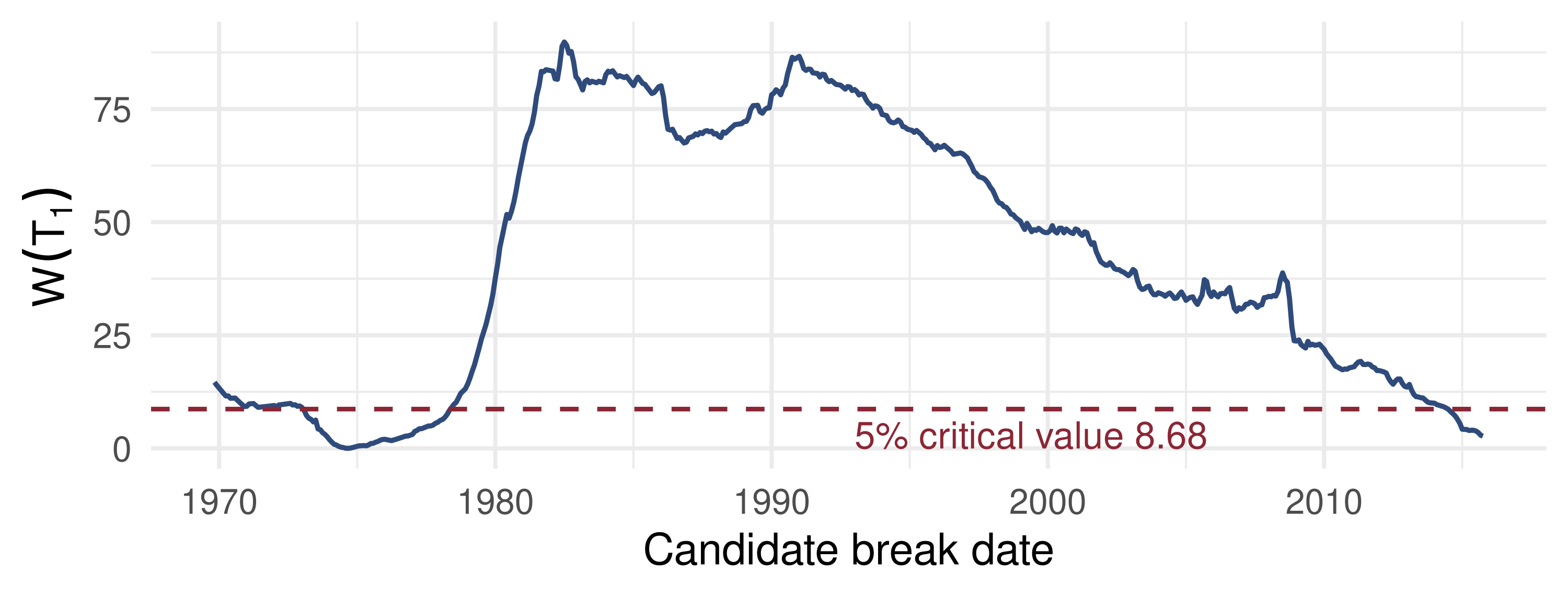
What the data say: sup-W rejects stability by a wide margin and puts the single break at mid-1982, the end of the Volcker disinflation; two breaks, August 1972 and July 1982, bracket a 1970s regime averaging 8.5% between two near 2.8%. The model fails in two places: the errors are autocorrelated, so the plain Wald overstates (the HAC version is far smaller, though still above 8.68), and the 2021–22 surge is too close to the end of the sample for a trimmed search to call it a regime.

📈 The Wald Path

\(W(T_1)\) over the middle 70% of the sample, from 1970 to 2015. Every date from 1979 on beats 8.68 by far. The dip in the mid-1970s is where a single split would leave high-inflation years on both sides; the peak, mid-1982, is the date that splits the sample best.

📉 CUSUM of Recursive Residuals

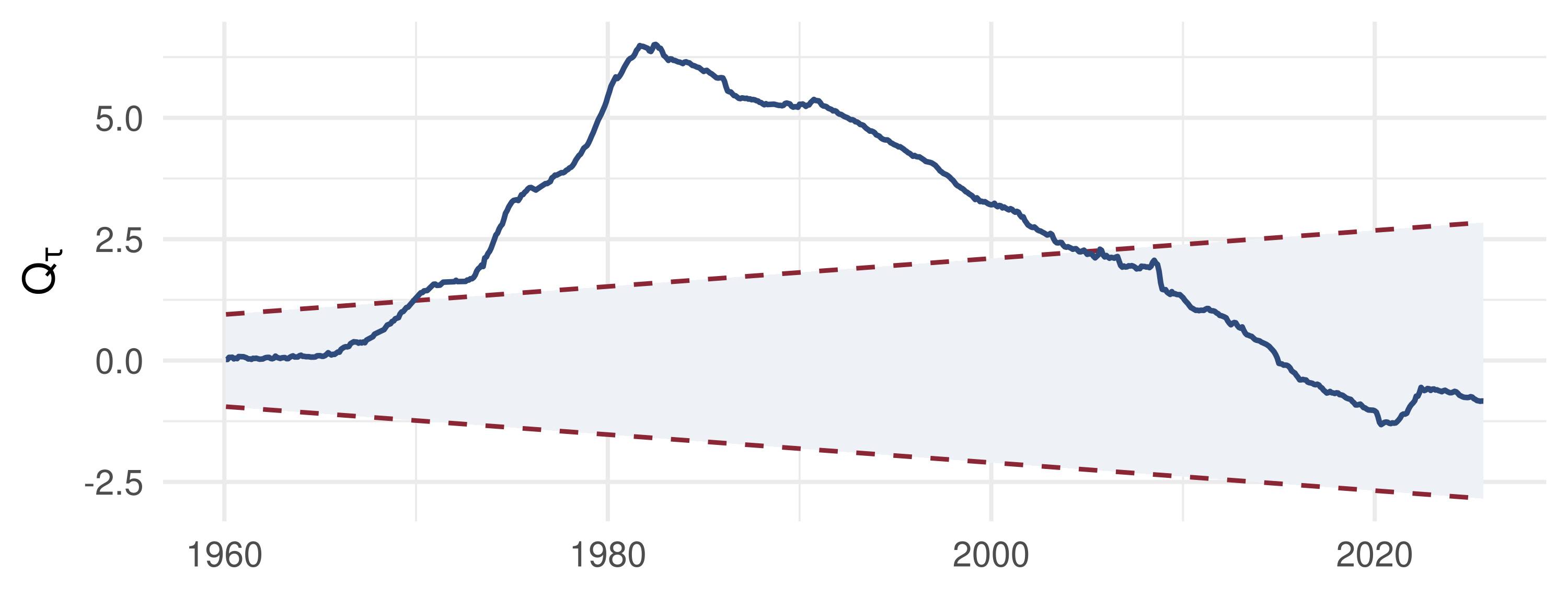
In the 1960s the forecasts from the running mean are too low month after month, so \(Q_\tau\) climbs and leaves the 5% band (dashed, \(\pm 0.948(1 + 2r)\)) at the end of 1969. One crossing is enough to reject stability. The path drifts back inside only in the mid-2000s, once the running mean has absorbed the 1970s.

📝 Quiz #1: Critical Values

You maximise the Wald statistic for a one-coefficient break over the middle 70% of the sample. At 5% you should compare \(\sup W\) with:

  • Andrews’ value, about 8.68
  • \(3.84\), the \(\chi^2_1\) value
  • \(1.96\), the normal value
  • \(1.358\), the Kolmogorov value

📝 Quiz #2: Bai–Perron

In the Bai–Perron framework, as \(T \to \infty\) with the break fraction fixed:

  • \(\hat T_1/T\) converges at rate \(T\), but \(\hat T_1 - T_1\) does not converge to zero
  • \(\hat T_1 \to T_1\), so the date is estimated exactly in large samples
  • \(\hat T_1/T\) converges at the usual rate \(\sqrt T\)
  • The slopes \(\hat\beta_j\) have a non-standard limit because the dates are estimated

📝 Quiz #3: CUSUM

The recursive CUSUM path stays inside the band \(\pm 0.948(1+2r)\) for the whole sample except for three consecutive months, where it pokes out. The conclusion at 5%:

  • Reject parameter stability
  • Do not reject: the path is inside 99% of the time
  • Reject only if the crossing lasts more than \(\pi T\) months
  • No conclusion without the break date

📋 Key Formulas

Known date \(W(T_1) \to \chi^2_k\)
Unknown date \(\sup_{\pi T \le T_1 \le (1-\pi)T} W(T_1) \to \sup_{\pi \le r \le 1-\pi} \frac{\lVert B(r) - rB(1)\rVert^2}{r(1-r)}\)
5% value 8.68 for \(k=1\), \(\pi=0.15\)
Bai–Perron \(\min \sum_j \sum_{t \in \text{regime } j}(y_t - x_t'\beta_j)^2\), \(\ T_j - T_{j-1} \ge \pi T\)
Rates \(\hat\lambda_j - \lambda_j = O_p(T^{-1})\), \(\ \hat T_j - T_j = O_p(1)\)
Sequential test \(\lim P\{F(\ell+1\mid\ell) \le x\} = G(x)^{\ell+1}\)
CUSUM \(Q_\tau = \frac{1}{\hat\sigma\sqrt{T-k}}\sum_{t=k+1}^\tau w_t \to B(r)\); \(\ b = 0.948(1+2r)\)
OLS-CUSUM \(\frac{1}{\hat\sigma\sqrt T}\sum_{t \le \tau}\hat e_t \to B(r) - rB(1)\); 5% value 1.358

📋 Summary

  • A break at a known date is a Chow–Wald test with a \(\chi^2_k\) limit
  • Searching over dates inflates the statistic: use Andrews’ sup-W critical values, and trim the ends
  • Bai–Perron estimate several dates by least squares; fractions are super-consistent, dates are not
  • The number of breaks is chosen sequentially, \(\ell\) against \(\ell+1\); with fixed size it is not consistent
  • CUSUM needs no alternative: cumulate recursive forecast errors and reject at the first crossing
  • US inflation: a high-inflation regime from 1972 to 1982 between two regimes near 2.8%

📚 Further Reading

  • Andrews (1993), Econometrica; Andrews (2003), Econometrica (critical values); Andrews & Ploberger (1994)
  • Bai & Perron (1998), Econometrica; Bai & Perron (2003), J. Applied Econometrics (computation)
  • Brown, Durbin & Evans (1975), JRSS B: recursive residuals and CUSUM
  • Ploberger & Krämer (1992), Econometrica: OLS-based CUSUM
  • Hansen (2001), J. Economic Perspectives: a non-technical survey; Perron (2006), in Palgrave Handbook of Econometrics

Next lecture: 17 · Realized Volatility, Durations, Direction and Value-at-Risk