Time Series Econometrics

Lecture 17: Realized Volatility, Durations, Direction and Value-at-Risk

Samir Orujov, PhD

Open lecture notes, after Stanislav Anatolyev’s course (2016)

🎬 The Idea in 3 Minutes

⬅ Previous lecture: 16 · Structural Breaks and Parameter Stability

A short film with the intuition. Watch it before the slides, or after. Captions: CC button.

🎯 Learning Objectives

By the end of this lecture, you will be able to:

• Distinguish observable, model-free volatility measures from model-based ones, and show that RiskMetrics is an IGARCH
• Explain why realized volatility converges to integrated volatility, and what microstructure noise does to it
• Write a multiplicative error model and the ACD model for durations
• Model the direction of change (autologit) and conditional quantiles (VaR, CAViaR)
• Backtest a VaR forecast with Kupiec’s test on real data

🔁 Warm-up from last time

You search over the middle 70% of the sample for one break in a mean and find \(\sup W = 7.9\). At 5%, what do you conclude?

• No evidence of a break: 7.9 is below Andrews’ critical value 8.68
• A break: 7.9 exceeds the \(\chi^2_1\) critical value 3.84
• A break, since the CUSUM test is never needed after sup-W
• Nothing can be said until the number of breaks is fixed

🗺️ Where We Are

Lecture 15 modelled the conditional variance \(\sigma_t^2\) with GARCH. Lecture 16 asked whether such parameters are stable.

\(\sigma_t^2\) is never observed: it exists only inside a model, and is only as good as the model’s mean and variance equations.

This last lecture asks three questions.

• Can volatility be measured rather than modelled?
• How do we model other positive quantities, such as the time between trades?
• How do we forecast what risk managers actually report: a quantile of tomorrow’s return?

❓ The Question

The number the regulator sees

Every day a bank reports its 1-day 99% Value-at-Risk: a loss it expects to exceed on only 1 day in 100. Every quarter the regulator counts the days on which the loss was larger.

Too many such days and the bank holds more capital. To get the count right the bank needs a good volatility measure, a good model of the tails, and a way to test its own quantile forecasts.

📐 Measures of Daily Volatility

Observable, model-free:

• \(|r_t|\) and \(r_t^2\): the earliest measures. \(E_{t-1}r_t^2 = \sigma_t^2\) when \(\mu_t = 0\), but a single squared return is very noisy
• JPMorgan’s RiskMetrics, an exponentially weighted average of past squared returns: \[RM_t = (1 - 0.94)\sum_{i=0}^{\infty} 0.94^{\,i}\, r_{t-i}^2\]

Not observable, model-based:

• \(\hat\sigma_t^2\) from an ARCH-type model. It is only as good as the model’s conditional mean and variance equations

📐 RiskMetrics Is an IGARCH

Split off the first term of the sum. With \(\lambda = 0.94\), \[\sigma_{t+1 \mid t}^2 = (1-\lambda)\sum_{i \ge 0}\lambda^i r_{t-i}^2 = (1-\lambda)\, r_t^2 + \lambda\,\sigma_{t \mid t-1}^2 .\]

This is GARCH(1,1) without a constant: \[\omega = 0, \qquad \alpha = 1 - \lambda = 0.06, \qquad \beta = \lambda = 0.94, \qquad \alpha + \beta = 1 .\]

• Integrated GARCH: shocks to the variance never die out, and there is no long-run level to revert to
• Nothing is estimated: \(\lambda = 0.94\) is fixed for all daily series
• Weights halve every \(\ln 0.5 / \ln 0.94 = 11.2\) days

📐 Realized Volatility

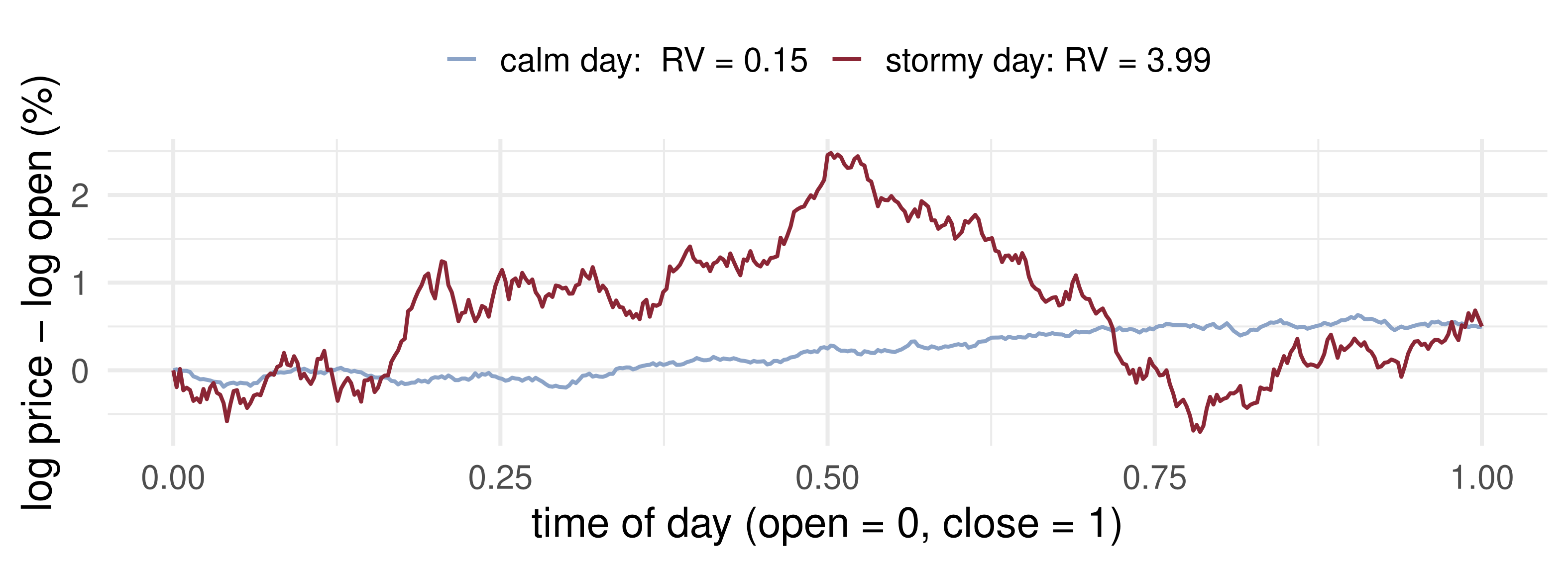
The daily return \(r_t = \log p_{\text{close}} - \log p_{\text{open}}\) sees only two prices. Very different intraday paths give the same \(r_t\).

Split day \(t\) into \(m\) intervals with intraday returns \(r_{t,i}\), \(i = 1, \dots, m\), and define \[RV_t = \sum_{i=1}^m r_{t,i}^2 \qquad \text{(Andersen, Bollerslev, Diebold and co-authors, 2000s).}\]

Like \(|r_t|\) and \(r_t^2\), it is observable and model-free. Unlike them, it is far less noisy, as the next two slides show.

📈 Same Return, Different Days

Both days open at 0 and close at \(+0.5\%\), so \(r_t = 0.5\) and \(r_t^2 = 0.25\) on each. The one-minute returns tell them apart: realized variance differs by a factor of about 25.

📐 Why Realized Volatility Works

Suppose the log price within the day follows \[d\log p_{t+s} = \mu_{t+s}\,ds + \sigma_{t+s}\,dW_{t+s}, \qquad s \in [0, 1],\] with \(\sigma^2_{t+s}\) the instantaneous volatility. Then as \(m \to \infty\) \[RV_t \xrightarrow{p} IV_t = \int_0^1 \sigma_{t+s}^2\,ds \qquad \text{(integrated volatility)},\] with a mixed-normal CLT at rate \(\sqrt m\).

• The drift \(\mu_{t+s}\) contributes only \(O(m^{-1})\) and can be neglected
• A GARCH, by contrast, must get the conditional mean right before its \(\hat\sigma_t^2\) means anything

📐 Covariance, Noise, and the Choice of \(m\)

Multivariate analogue. For a vector of intraday returns, the realized covariance matrix \[RC_t = \sum_{i=1}^m r_{t,i}\, r_{t,i}' .\]

But \(m\) is finite, and one would like it large. At very high frequencies prices bounce between bid and ask, and ticks are discrete. This market microstructure noise adds a term to every \(r_{t,i}^2\), and the bias grows with \(m\).

In practice the sampling interval is about 5 to 15 minutes: fine enough for \(RV_t\) to be precise, coarse enough for the noise to be small.

💻 Noise and the Sampling Frequency

set.seed(2026)
n_sec <- 23400; days <- 200; s <- (1:n_sec) / n_sec
sig <- 0.01 * sqrt(0.6 + 3.2 * (s - 0.5)^2)                    # U-shaped intraday vol
IV <- mean(sig^2)                                              # integrated variance per day
grid <- c(13, 26, 78, 390, 1170, 4680, 23400)                  # 30 min ... 1 second
res <- replicate(days, {
  lp <- cumsum(sig * rnorm(n_sec) / sqrt(n_sec))               # efficient log price
  obs <- lp + rnorm(n_sec, 0, 0.0001)                          # + noise, 1 basis point
  sapply(grid, function(m) { k <- seq(n_sec / m, n_sec, by = n_sec / m)
    c(clean = sum(diff(c(0, lp[k]))^2), noisy = sum(diff(c(0, obs[k]))^2)) })
})
round(cbind(m = grid, clean = rowMeans(res[1, , ]) / IV, noisy = rowMeans(res[2, , ]) / IV), 2)

         m clean noisy
[1,]    13  1.01  1.01
[2,]    26  1.00  1.01
[3,]    78  0.99  1.01
[4,]   390  1.00  1.09
[5,]  1170  1.00  1.27
[6,]  4680  1.00  2.08
[7,] 23400  1.00  6.39

Average \(RV_t / IV_t\) over 200 simulated days. Without noise it is 1 at every \(m\). With a one-basis-point noise, it is fine at 5 minutes (\(m = 78\)) and more than six times too large at one second.

📐 Multiplicative Error Models

Many quantities in finance are positive: \(RV_t\), the daily range, \(|r_t|\), and the durations \(d_t = t_i - t_{i-1}\) between transactions. Durations cluster: busy periods have short gaps.

MEM (Engle, 2002)

\[x_t = \psi_t\,\varepsilon_t, \qquad \psi_t = E_{t-1}x_t, \qquad \varepsilon_t \sim \text{iid } \mathcal D(1),\ \ \varepsilon_t > 0,\ E\varepsilon_t = 1 .\]

It is the positive analogue of \(r_t = \sigma_t\eta_t\), \(\eta_t \sim (0, 1)\): there the shock scales a standard deviation, here it scales a mean.

📐 The ACD Model

For durations, Engle & Russell (1998): Autoregressive Conditional Duration, \[d_t = \psi_t\varepsilon_t, \qquad \text{ACD}(1,1):\ \ \psi_t = \omega + \alpha\, d_{t-1} + \beta\,\psi_{t-1}, \qquad \omega > 0,\ \alpha, \beta \ge 0,\] with \(\alpha + \beta < 1\) for a finite unconditional mean duration \(\omega/(1-\alpha-\beta)\).

Choice of \(\mathcal D\)	Method	Analogue in GARCH
Standard exponential	QMLE, \(\ell_t = -\log\psi_t - d_t/\psi_t\)	Gaussian QMLE
Weibull\((\lambda)\), Burr\((\lambda, \mu)\)	MLE	Student-\(t\) MLE

The exponential QMLE is consistent whenever \(\psi_t\) is correctly specified, whatever the true \(\mathcal D\).

📐 Beyond Mean and Variance

So far dynamic models have targeted

• ✓ the conditional mean (ARMA, VAR, TAR)
• ✓ the conditional variance (GARCH, SV, RV)
• ✓ the conditional density: conditional skewness and kurtosis (ARCD)

Two more objects are often what a user actually needs:

• the direction of tomorrow’s move, \(\mathbb 1\{r_t > 0\}\)
• a quantile of tomorrow’s return: Value-at-Risk

📐 Direction of Change: Autologit

The sign indicator has conditional mean equal to a conditional probability: \[E_{t-1}\,\mathbb 1\{r_t > 0\} = \Pr_{t-1}\{r_t > 0\}.\]

Autologit(1,1): \[\Pr_{t-1}\{r_t > 0\} = \frac{1}{1 + \exp\{-w_t\}}, \qquad w_t = \varphi + \alpha\,\mathbb 1\{r_{t-1} > 0\} + \gamma\, r_{t-1} + \beta\, w_{t-1} .\]

• \(w_t\) plays the role of \(\sigma_t^2\) in GARCH: a recursion driven by yesterday’s data and its own lag
• Estimated by maximum likelihood with the Bernoulli likelihood \(\sum_t \big[\mathbb 1\{r_t>0\}\log P_t + \mathbb 1\{r_t \le 0\}\log(1 - P_t)\big]\)

📐 Conditional Quantiles: Value-at-Risk

Value-at-Risk

The \((1-p)\cdot 100\%\) VaR is the conditional \(p\)-quantile of the return: \[\Pr_{t-1}\big\{r_t \le \mathrm{VaR}_t\big\} = p .\]

Indirect modelling. If \((r_t - \mu_t)/\sigma_t = \eta_t \sim \text{iid } \mathcal D(0, 1, \vartheta)\), estimate \(\hat\mu_t\), \(\hat\sigma_t\) and the density \(\hat f_{\mathcal D}\), then \[\widehat{\mathrm{VaR}}_t = \hat\mu_t + \hat\sigma_t\, q_p\big(\hat f_{\mathcal D}\big),\] with \(q_p\) the \(p\)-quantile of the fitted standardised distribution. Normal: \(q_{0.01} = -2.326\), \(q_{0.05} = -1.645\).

📐 Direct Modelling: CAViaR

Model the quantile itself, with no distribution (Engle & Manganelli, 2004): \[r_t = q_t^p + e_t, \qquad \text{Quantile}_p\big(e_t \mid I_{t-1}\big) = 0,\] \[q_t^p = \omega + \beta\, q_{t-1}^p + \alpha\, g(r_{t-1}), \qquad \text{e.g. } g(r) = |r| .\]

Estimate by quantile regression: minimise \[\sum_t \rho_p\big(r_t - q_t^p\big), \qquad \rho_p(u) = u\,\big(p - \mathbb 1\{u < 0\}\big).\]

The check function \(\rho_p\) penalises a return below the quantile with weight \(1-p\) and one above it with weight \(p\); its minimiser is the \(p\)-quantile.

🧪 Backtesting a VaR

Define the hit \(I_t = \mathbb 1\{r_t < \widehat{\mathrm{VaR}}_t\}\). If the VaR is correct, the hits are iid Bernoulli(\(p\)). With \(x\) hits in \(n\) days and \(\hat\pi = x/n\), Kupiec’s unconditional-coverage test is \[LR_{uc} = -2\log\big[(1-p)^{n-x}p^{x}\big] + 2\log\big[(1-\hat\pi)^{n-x}\hat\pi^{x}\big] \xrightarrow[H_0]{d} \chi^2_1 .\]

• Reject at 5% if \(LR_{uc} > 3.84\): too many hits or too few
• Christoffersen (1998) adds a test that the hits are independent: clustered hits mean the VaR reacts too slowly

Not in the 2016 notes: added from Kupiec (1995) and Christoffersen (1998).

✏️ Worked Example: RiskMetrics VaR

Yesterday \(\sigma_{t \mid t-1}^2 = 1.20\) (\(\%^2\)) and the index fell \(r_t = -2.5\%\). A fund holds 10 million USD.

1. Update. \(\sigma_{t+1 \mid t}^2 = 0.06 \times 6.25 + 0.94 \times 1.20 = 0.375 + 1.128 = 1.503\), so \(\sigma_{t+1 \mid t} = 1.226\%\).

2. VaR at 99%. \(\mathrm{VaR}_{t+1} = -2.326 \times 1.226 = -2.85\%\): a loss above 285,000 USD on 1 day in 100.

✏️ Worked Example: Backtesting It

Over \(n = 1000\) days the same VaR is exceeded \(x = 18\) times, against \(10\) expected. So \(\hat\pi = 0.018\) and

\[\begin{aligned} LR_{uc} &= -2\,[982 \ln 0.99 + 18 \ln 0.01] + 2\,[982 \ln 0.982 + 18 \ln 0.018] \\ &= 185.53 - 180.30 = 5.23 > 3.84 . \end{aligned}\] Reject: the VaR is exceeded too often. With 6 hits instead, \(LR_{uc} = 1.89\): fewer hits than expected, but not significantly so.

🧠 Think-Pair-Share

1. A colleague writes RiskMetrics as \(\sigma_t^2 = \omega + \alpha r_{t-1}^2 + \beta\sigma_{t-1}^2\) with \(\alpha = 0.94\). What should \(\omega\), \(\alpha\), \(\beta\) be? Is the model covariance stationary?

2. A bank’s 99% VaR was exceeded on 4 of the last 250 days. Does Kupiec’s test reject?

3. Why is it hopeless to backtest a 99% VaR on one month of data?

✅ Think-Pair-Share: Solution

1. \(\omega = 0\), \(\alpha = 1 - \lambda = 0.06\), \(\beta = \lambda = 0.94\). Since \(\alpha + \beta = 1\) it is an IGARCH: not covariance stationary, and there is no unconditional variance.

2. \(\hat\pi = 0.016\) and \[\begin{aligned} LR_{uc} &= -2[246\ln 0.99 + 4\ln 0.01] + 2[246\ln 0.984 + 4\ln 0.016] \\ &= 41.79 - 41.02 = 0.77 < 3.84 . \end{aligned}\] No rejection: 4 hits against 2.5 expected is within sampling error.

3. In 21 days the expected number of hits is \(0.21\). Zero hits has probability 0.81 if the VaR is right, and remains likely if it is badly wrong, so the test has almost no power.

🎛️ Explore: The RiskMetrics Decay \(\lambda\)

viewof lam = {
  const input = Inputs.range([0.80, 0.995], {value: 0.94, step: 0.005, label: "λ (decay)"});
  ['pointerdown','touchstart','mousedown','click','wheel','pointermove','touchmove']
    .forEach(e => input.addEventListener(e, ev => ev.stopPropagation()));
  return input;
}

ewma = {
  const r = ret, n = r.length, out = [];
  let s2 = r.slice(0, 60).reduce((a, b) => a + b * b, 0) / 60, hits = 0, cnt = 0;
  for (let t = 1; t < n; t++) {
    s2 = lam * s2 + (1 - lam) * r[t - 1] ** 2;
    const v = -2.326 * Math.sqrt(s2);
    const hit = t >= 250 && r[t] < v;
    if (t >= 250) { cnt++; if (hit) hits++; }
    out.push({t, r: r[t], v, hit});
  }
  const p = 0.01, ph = hits / cnt;
  const LR = -2 * ((cnt - hits) * Math.log(1 - p) + hits * Math.log(p))
             + 2 * ((cnt - hits) * Math.log(1 - ph) + hits * Math.log(ph));
  return {out, hits, cnt, LR};
}

Plot.plot({
  width: 1100, height: 300, marginLeft: 70, marginBottom: 50, marginTop: 30,
  style: {fontSize: "18px"},
  x: {label: "trading day since Oct 2016"}, y: {label: "return (%)", domain: [-13, 10], grid: true},
  marks: [
    Plot.lineY(ewma.out, {x: "t", y: "r", stroke: "#c9d4e6", strokeWidth: 1}),
    Plot.lineY(ewma.out, {x: "t", y: "v", stroke: "#2f4b7c", strokeWidth: 2}),
    Plot.dot(ewma.out.filter(d => d.hit), {x: "t", y: "r", r: 4, fill: "#8b2635"})
  ]
})

html`<div style="font-size:28px">Blue: normal 99% VaR. Red: hits. ${ewma.hits} hits in ${ewma.cnt} days (${(100 * ewma.hits / ewma.cnt).toFixed(2)}%, expected 1%) · Kupiec LR = ${ewma.LR.toFixed(1)} ${ewma.LR > 3.84 ? "· reject" : "· do not reject"}</div>`

💰 Case Study: Backtesting S&P 500 VaR

📈 The question

Three ways to forecast tomorrow’s 1% and 5% quantile of the S&P 500 return.

1. Does RiskMetrics with normal quantiles pass Kupiec’s test?
2. Does model-free historical simulation do better?
3. Does replacing the normal quantile by the empirical one (indirect modelling with \(\hat f_{\mathcal D}\)) fix the tails?

📊 The data

Series: S&P 500 close, FRED SP500

Period: Oct 2016 – Oct 2026; VaR evaluated on the last 2,261 days

Transformation: \(r_t = 100\,\Delta\log P_t\); \(\mu_t = 0\); first 250 days used only to start the forecasts

sp <- read.csv("https://fred.stlouisfed.org/graph/fredgraph.csv?id=SP500")

💰 Case Study: Hit Rates and Kupiec

r <- r_all; n <- length(r); ev <- 251:n
s2 <- numeric(n); s2[1] <- mean(r[1:60]^2)
for (t in 2:n) s2[t] <- 0.94 * s2[t - 1] + 0.06 * r[t - 1]^2      # sigma^2_{t|t-1}
z <- r / sqrt(s2)                                                  # standardised returns
kupiec <- function(hit, p) { x <- sum(hit); m <- length(hit); ph <- x / m
  LR <- -2 * ((m - x) * log(1 - p) + x * log(p)) + 2 * ((m - x) * log(1 - ph) + x * log(ph))
  c(hit_rate = 100 * ph, LR = LR, p_value = pchisq(LR, 1, lower.tail = FALSE)) }
var_fc <- function(p) list(
  RiskMetrics_normal = qnorm(p) * sqrt(s2[ev]),
  historical_250d    = sapply(ev, function(t) quantile(r[(t - 250):(t - 1)], p)),
  filtered_HS        = sapply(ev, function(t) sqrt(s2[t]) * quantile(z[1:(t - 1)], p)))
V1 <- var_fc(0.01); V5 <- var_fc(0.05)
round(rbind(t(sapply(V1, function(v) kupiec(r[ev] < v, 0.01))),
            t(sapply(V5, function(v) kupiec(r[ev] < v, 0.05)))), 3) |>
  `rownames<-`(paste(rep(c("1%:", "5%:"), each = 3), names(V1)))

                       hit_rate     LR p_value
1%: RiskMetrics_normal    2.344 29.936   0.000
1%: historical_250d       1.681  8.785   0.003
1%: filtered_HS           0.929  0.119   0.731
5%: RiskMetrics_normal    5.750  2.557   0.110
5%: historical_250d       5.484  1.084   0.298
5%: filtered_HS           5.838  3.180   0.075

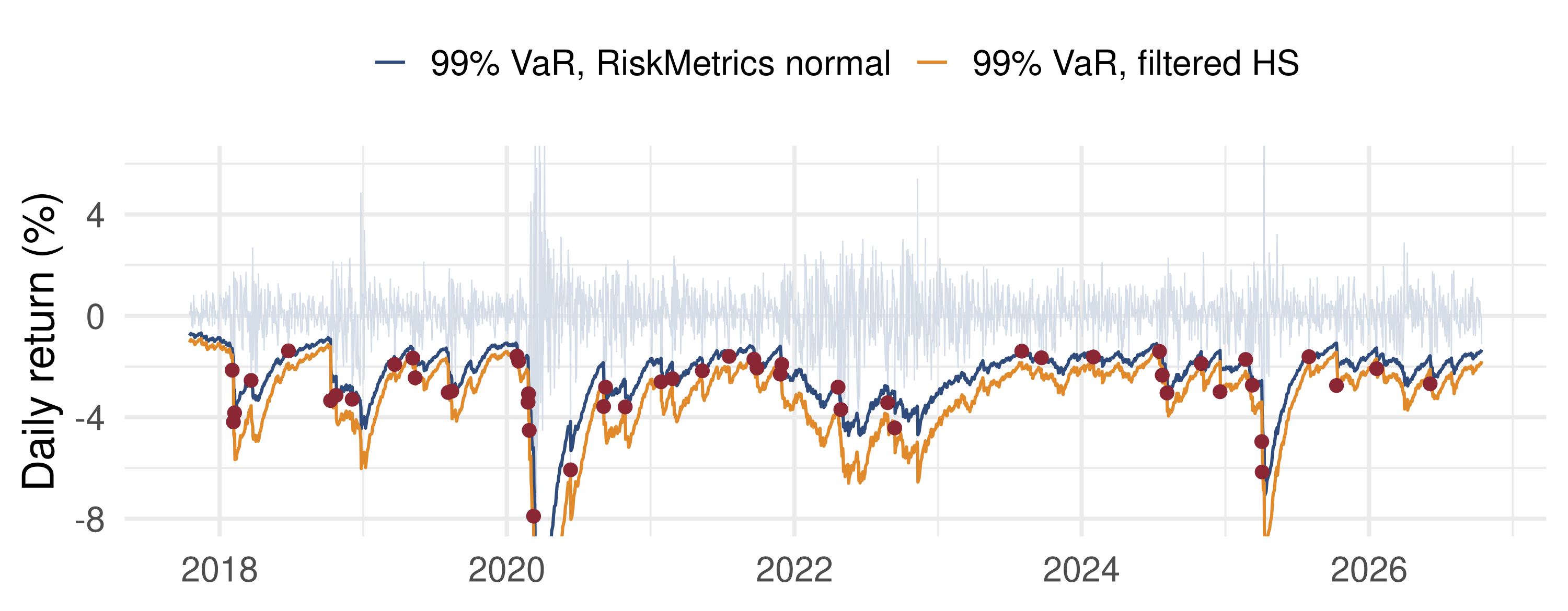
Hit rates in %, against 1 and 5. Read the 1% rows first.

💰 Case Study: The Normal Tail Fails

What the data say: at 5% all three forecasts pass. At 1% the normal RiskMetrics VaR is exceeded on 2.3% of days (red dots), and Kupiec rejects decisively; historical simulation, which reacts slowly, is also rejected. Keeping RiskMetrics for \(\sigma_t\) but taking the quantile from the standardised returns passes. The failure is the normal tail, not the volatility model.

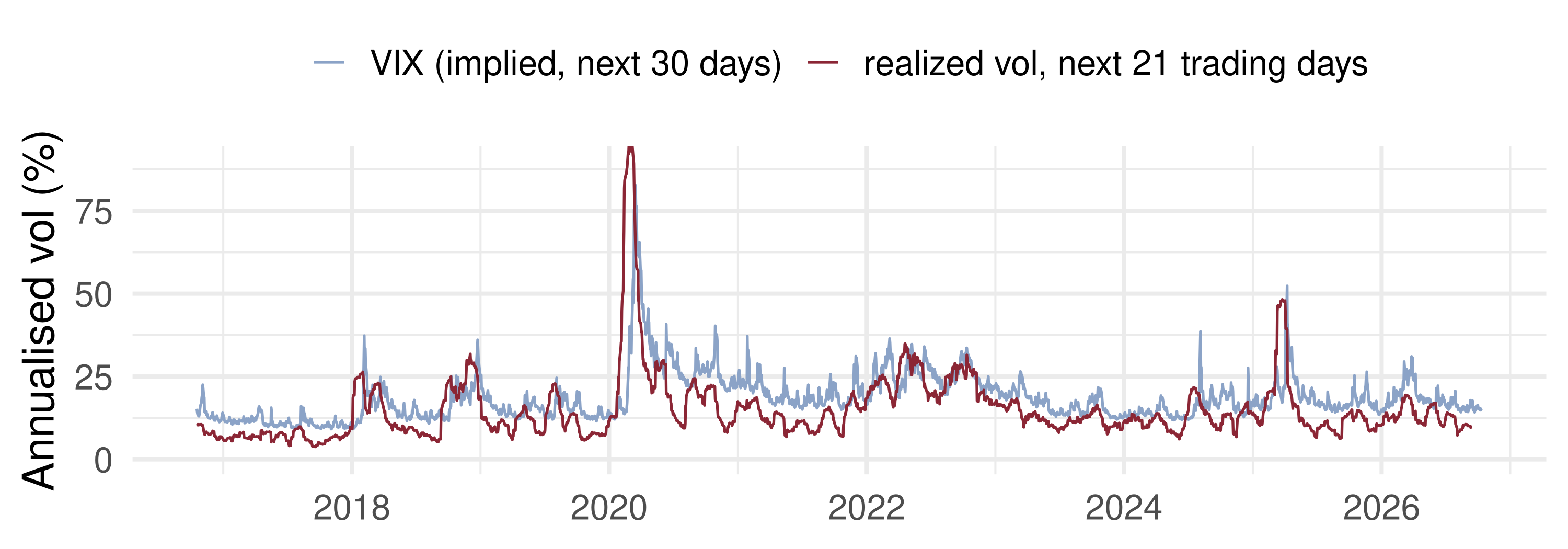
📈 VIX: Volatility Looking Forward

The VIX is the volatility priced into one-month S&P 500 options, a risk-neutral expectation: forward-looking, but not a forecast under the real-world measure. It averages 18.7% against 15.0% realized, and exceeds realized vol on 84% of days: investors pay a variance risk premium. Its correlation with future realized vol is 0.60, against 0.50 for the backward-looking RiskMetrics.

📝 Quiz #1: RiskMetrics

RiskMetrics with \(\lambda = 0.94\) is a GARCH(1,1) with

• \(\omega = 0\), \(\alpha = 0.06\), \(\beta = 0.94\)
• \(\omega = 0\), \(\alpha = 0.94\), \(\beta = 0.06\)
• \(\omega = 0.06\), \(\alpha = 0.94\), \(\beta = 0\)
• \(\omega > 0\) estimated from the data, \(\alpha + \beta = 0.94\)

📝 Quiz #2: Realized Volatility

Why do practitioners compute \(RV_t\) from 5-minute returns rather than from every tick?

• Microstructure noise inflates RV at very high frequencies
• Because \(RV_t\) diverges as \(m \to \infty\) even without noise
• Because the drift term dominates at high frequency
• Because tick data are not observable

📝 Quiz #3: Backtesting

A 95% VaR is exceeded on 0 of 500 days. Kupiec’s test:

• Rejects: 0 hits is far fewer than the 25 expected, so the VaR is too conservative
• Does not reject: no hits is the best possible outcome
• Cannot be computed, because \(\log \hat\pi\) is undefined
• Rejects only if the hits are clustered

📋 Key Formulas

RiskMetrics	\(\sigma^2_{t+1\mid t} = 0.06\,r_t^2 + 0.94\,\sigma^2_{t\mid t-1}\), an IGARCH
Realized volatility	\(RV_t = \sum_{i=1}^m r_{t,i}^2 \to IV_t = \int_0^1\sigma^2_{t+s}\,ds\)
MEM / ACD(1,1)	\(x_t = \psi_t\varepsilon_t\), \(E\varepsilon_t = 1\); \(\ \psi_t = \omega + \alpha d_{t-1} + \beta\psi_{t-1}\)
Autologit(1,1)	\(P_t = 1/(1+e^{-w_t})\), \(\ w_t = \varphi + \alpha\mathbb 1\{r_{t-1}>0\} + \gamma r_{t-1} + \beta w_{t-1}\)
VaR, indirect	\(\widehat{\mathrm{VaR}}_t = \hat\mu_t + \hat\sigma_t q_p(\hat f_{\mathcal D})\)
CAViaR	\(q_t^p = \omega + \beta q_{t-1}^p + \alpha|r_{t-1}|\), \(\ \min\sum_t\rho_p(r_t - q_t^p)\)
Kupiec	\(LR_{uc} = -2\log[(1-p)^{n-x}p^x] + 2\log[(1-\hat\pi)^{n-x}\hat\pi^x] \to \chi^2_1\)

📋 Summary

• \(|r_t|\), \(r_t^2\) and RiskMetrics are observable and model-free; GARCH \(\hat\sigma_t^2\) is model-based
• RiskMetrics is an IGARCH with \(\omega = 0\), \(\alpha = 0.06\), \(\beta = 0.94\)
• Realized volatility converges to integrated volatility; noise sets the sampling interval at 5–15 minutes
• MEM and ACD model positive series as a conditional mean times a unit-mean shock
• Direction (autologit) and quantiles (VaR, CAViaR) are dynamic models in their own right
• On the S&P 500 the 99% normal VaR fails Kupiec’s test; the tail, not the volatility, is the problem

📚 Further Reading

• J.P. Morgan/Reuters (1996), RiskMetrics — Technical Document
• Andersen, Bollerslev, Diebold & Labys (2003), Econometrica; Barndorff-Nielsen & Shephard (2002), JRSS B
• Engle & Russell (1998), Econometrica: ACD; Engle (2002), J. Applied Econometrics: MEM
• Engle & Manganelli (2004), JBES: CAViaR; Kupiec (1995), J. Derivatives; Christoffersen (1998), IER
• Tsay (2010), ch. 3, 5 and 7

This is the last lecture of the course.